Introduction
A total of 36.8% of the land area worldwide is agricultural land (FAO, 2019). Agriculture has been developed for more than a thousand years, and agricultural ecosystems are a unique landscape that provides food but is disturbed by human activity. This disturbance can strongly affect biodiversity and the environment (McLaughlin & Mineau, 1995). Inappropriate cultivation and agricultural management practices and chemical materials such as herbicides and fertilizers can also reduce biodiversity (Dudley & Alexander, 2017), leading to a decrease in ecosystem service value through landscape simplification, soil degradation, water pollution, poor water and soil conservation, and the extinction of species (Kanianska, 2016). The overuse of agricultural chemicals can change the species composition of agricultural ecosystems and negatively affect the gene pool by reducing the number of natural enemies and increasing pests’ and weeds’ drug resistance (Bueno et al., 2017; Cloyd, 2012). These factors decrease agricultural sustainability and biodiversity.
Agricultural practices that not only produce high quantities of food but also balance biodiversity and environmental friendliness are crucial. Benton et al. (2003) described the crucial nature of identifying methods to mitigate the negative effects of agriculture on the biodiversity of various ecosystems. Because long-term agricultural activity reduces the biodiversity in farmland plants directly and indirectly (Stehlik et al., 2007; Vickery et al., 2001), many studies have indicated that the boundaries of seminatural habitat farmlands are an essential dispersal corridor for fauna (Dennis & Gary, 1992). The vegetation in seminatural habitat farmlands comprises natural, human-made and mixed planting systems. Seminatural habitat farmlands maintain wild plant biodiversity as well as the variety in structure in trees, shrubs, grasslands, and weeds. The variety of structure determines the diversity of function, ensures the protection of the natural enemies of pests, and decreases the number of pest species. Altieri (1984) indicated that planting brussels sprouts (Brassica oleracea L. var. gemmifera) with broad beans (Vicia faba L.) and field mustard (Brassica kaber [DC] L.C. Wheeler) deters pests more than does planting brussels sprouts alone. Lagerlof and Wallin (1993) noted that in terms of the plant biodiversity in the borderlines of farmlands, higher bank plant biodiversity results in more species of pests in larger quantities. Wyss (1996) revealed that if apple orchards are human-made bands of grassland 1 m apart, the number of natural enemies of aphids increase. The results of Yu et al. (1996) indicated that several flowers in nonpaddy habitats and Poaceae weeds are crucial to protecting natural enemies.
Most of the agricultural landscapes consist of farmlands; buildings such as greenhouses, farmhouses, and warehouses; and seminatural habitats at the borders of farmlands such as grasslands, ponds, forests, and brooks. These habitats are crucial to habitants even if they are small (Jobin et al., 2001; Morandin & Winston, 2014). The borders of agricultural landscapes are mostly human made. If landscape elements such as flora and native plant species are predominant, the landscapes can be artificially reconfigured with ease to create an agricultural ecosystem that balances biodiversity and ecofriendliness. In such an ecosystem, the cultivated areas and various bands of farmland vegetation serve as habitats for the native fauna and flora (Marshall & Moonen, 2002).
The scope of farmland landscape in Taiwan is extensive. Although the types of landscapes, flora, landforms, and land use in farmlands are less varied than in the natural environment, the time for basic investigation and research can be several years and require considerable costs, labor, and material resources. To efficiently utilize funding and resources, the research production value must be calculated, researchers must be allocated tasks, the progress and outcome must be periodically evaluated, and the format and method for sharing data must be determined. Therefore, developing and evaluating plant species investigation methods that involve biogeographical scales (Kent & Coker, 1992) are essential to research.
Wu et al. (2008) indicated that the regional grass flora investigation in Taiwan requires at least 6.1 random quadrats with an area of 1×1 m2. However, the scale of the investigation was the entire Taiwan, and the scope of agriculture was defined as all activity on farmlands, banks, and orchards. Therefore, to identify the types of weeds in farmlands, investigating the grass management, microhabitat conservation, and agricultural landscape creation is insufficient; the category of “farmland” must be subdivided. We investigated the plants in the agricultural ecosystems in Taiwan during the most appropriate seasons for the sake of efficiency and developed a methodology for evaluating agricultural ecosystem services.
Materials|Methods
Study sites
We began the ground cover plant investigation at long-term agricultural ecology research stations located in the center of Taiwan, where the average annual temperature is 22-25.5°C and annual precipitation is 900-3,000 mm (Center Weather Bureau Data, 1971-2020). The study sites were Chi-Ko Branch Farm (CK site), Yuin-Lin Branch Station (YL site), Chia-Yi Agricultural Experiment Branch (CY site), Gu-Keng Branch Farm (GK site), and two tea gardens in Min-Jian (MJ site), one practicing conventional farming and one sustainable farming (MJ-CF and MJ-SF sites) (Fig. 1). The crops in each site are as follows: rice and peanuts at the CK and YL sites, lychee at the CY and GK sites, and tea at the MJ-CF and MJ-SF sites. Weed management comprises regular mowing and use of herbicides at the CK, YL, and MJ-CF sites and regular mowing alone at the CY, GK, and MJ-SF sites.
Field investigation
The investigation was conducted from 2017 to 2020 during spring (March to May), summer (June to August), autumn (September to November), and winter (December to February). The habitats investigated were farmlands (CK & YL sites), banks (CK & YL sites), orchards (CY & GK sites), and tea gardens (MJ-CF & MJ-SF sites). In accordance with the recommendations of Wu et al. (2008), more than 10 random quadrats with an area of 1×1 m2 in different habitats of the sites were investigated. The coordinates, altitudes, and vertical projection cover of the quadrats and the scientific names of the species were documented. If the roots of a plant were outside the quadrat but its branches or leaves were inside, the plants were considered inside the quadrat. Because vertical projection cover was examined, the total plant cover could be more than 100% in each sample.
Data analysis
Cluster analysis was performed to group the habitats with similar plant composition in each quadrat, and the data were combined into clusters using R (version 4.1.1; The R Foundation for Statistical Computing, Vienna, Austria). After cluster analysis, individual quadrats were randomly selected to calculate the number of plant species for each cluster and season. We then merged the data with those of nearby quadrats and calculated the number of plant species to create species–area curves by plotting the total number of species in each season. The species–area curves were created using Microsoft Excel (version 2013; Microsoft, Redmond, WA, USA), and the point of tangency was set to a slope of 1 to identify areas in which the number of species increased slowly; the point of tangency represents the minimum number of samples. For habitats in the same cluster, one-way analysis of variance was performed using JMP (version 6.0; Statistical Discovery, SAS Institute, Cary, NC, USA) to identify differences in cover and number of species among the habitats and seasons and to determine the ideal sampling season.
Results
The habitats in each site were divided into five clusters: 1) the farmland cluster (F cluster), comprising farmland data from the CK and YL sites; 2) the bank cluster (B cluster), comprising bank data from the CK and YL sites; 3) the Chia-Yi orchard cluster (CY-O cluster), comprising orchard data from the CY site; 4) the Gu-Keng orchard cluster (GK-O cluster), comprising orchard data from the GK site; and 5) the tea garden cluster (T cluster), comprising tea garden data from the MJ-CF and MJ-SF sites (Fig. 2). The data from the CK-F and YL-F clusters revealed two independent monophyletic groups in the F cluster. The data from the MJ-CF and MJ-SF clusters revealed two independent monophyletic groups in the T cluster. However, because the data from the CK-B and YL-B clusters were scattered, we did not mark them in Fig. 2.
Fig. 3 illustrates the species–area curves for the clusters and seasons. The number of quadrats in each cluster was as follows: 3.9-9.4 in the F cluster, 8.9-11.2 in the B cluster, 13.2-18 in the CY-O cluster, 10.3-14.9 in the GK-O cluster, and 5.3–8.1 in the T cluster. Minimum quadrats for weed investigation in agricultural ecosystem for each microhabitat were presented in Table 1.
Table 2A presents a comparison of the number of plant species among the clusters. The GK-O cluster had the most species during all four seasons, followed by the CY-O, T, B, and F clusters. Significant differences in number of plant species were observed in the F, B, CY-O, and GK-O clusters. The F cluster had the most species in autumn, followed by in winter, summer, and spring. The B cluster had the most species in spring, followed by in summer, autumn, and winter. The CY-O cluster had the most species in spring, followed by in autumn, winter, and summer. The GK-O cluster had the most species in spring, followed by in summer, autumn, and winter. No significant differences in number of plant species among the four seasons were observed in the T cluster.
Table 2B presents a comparison of plant cover among the clusters. The GK-O cluster had the highest cover in all four seasons, followed by the CY-O, T, B, and F clusters. Significant differences in plant cover among the seasons were observed. The F cluster had the highest cover in spring and autumn, followed by in summer and winter. The B cluster had the highest cover in summer and autumn, followed by in spring and winter. The CY-O cluster had the highest cover in autumn and winter, followed by in spring and summer. The GK-O cluster had the highest cover in summer and autumn, followed by in spring and winter. The T cluster had the highest cover in summer, followed by in autumn, spring, and winter.
Discussion
Our results in comparison with those of Wu et al. (2008) indicate that 6.1 random 1×1 m2 quadrats are insufficient for a plant survey in the microhabitats of the agricultural ecosystem. For areas such as paddy fields and tea gardens with short, high-cover plants, such as peanuts, 10 (>9.4) quadrats should be used in each season. For habitats on the boundaries of farmlands, such as banks, 12 (>11.2) quadrats should be used in each season. For orchard clusters with tall plants and cultivated grasslands, 18 quadrats should be used to determine the number of plant species number in the agricultural areas (Table 1).
All clusters except the F cluster had the most species during spring (Table 2A). This is probably because the temperature in spring increases, causing seeds to germinate and resulting in a large number of species but low plant cover. In Taiwan, pre-emergency herbicides are applied to paddy fields such as those in the F cluster to inhibit the germination and growth of weeds and prevent a population from being established before rice transplanting (January to February). After the first harvest, farming transitions from paddies to upland fields. After the cultivation of peanut in autumn, the number of plant species increases considerably because of irrigation. However, the unique paddy–upland crop rotation to deter disease, pests, and weeds during rice cultivation in Asian monsoon areas strongly affects soil microhabitats and reduces weed biodiversity (Hsiao et al., 2013). Therefore, the number of plant species in such areas is small.
The results for plant cover indicate normal plant growth conditions, and the highest growth period, producing a dense canopy, is from summer to autumn. For the F cluster, the highest growth period was spring and autumn (Table 2B). This can probably be attributed to the fact that during rice harvest in June and July, the above-ground plants are removed, reducing plant cover. Overall, summer and autumn are conducive to investigating plant cover in agricultural ecosystems. The accumulation of soil organic carbon (SOC) is caused by interaction among dynamic ecological processes such as photosynthesis, decomposition, and soil respiration (Ontl & Schulte, 2012) and is directly or indirectly affected by the formation of soil organic matter after plant decomposition. Large amounts of SOC in plant biomass (Conant et al., 2017) is directly reflected by above-ground cover. In light of farmland carbon rights, plant biomass will become a crucial indicator.
Investigations of plant ground cover can be conducted throughout the year with at least 18 quadrats in the subdivided microhabitats. However, if human and material resources are limited, 10 quadrats should be the minimum for farmlands in autumn and for the other microhabitats in spring. The minimum number of quadrats is 10 for banks, 17 for orchards, and 9 for tea gardens.
Acknowledgments
This work would not have been possible without the assistance of the site manager and technicians, Dr. Jer-Way Chang, Dr. Dah-Jing Liao, Mr. Rei-Chang Wang, Mr. Chin-Shing Chang, Mr. Ru-Hong Lin, Mr. Jin-Cheng Hsu, Mr. Ching-Rong Chang, Mr. Hong-Mou Chang, and Ms. Hsiu-Jeng Liu. We are grateful to the owners of the conventional and organic tea gardens, Mr. Wen-Feng Chen and Mr. Mu-Ton Chang, who allowed us to study their gardens. We also appreciate Miss Ya-Hui Shih and Ms. Li-Xiang Zhang, who assisted in the data analysis. This manuscript was edited by Wallace Academic Editing.
References
FAO (Food and Agriculture Organization of the United Nation) (2019, Retrieved January 17, 2022) FAO Statistical Databases from http://www.fao.org/faostat/en/#data/RL/visualize
Figures and Tables
Fig. 1
Locations of long-term agricultural ecological research. CK, Chi-Ko Branch Farm; YL, Yuin-Lin Branch Station; CY, Chia-Yi Agricultural Experiment Branch Farm; GK, Gu-Keng Branch Farm; MJ-CF, Min-Jian tea garden for conventional farming; MJ-SF, Min-Jian tea garden for sustainable farming.
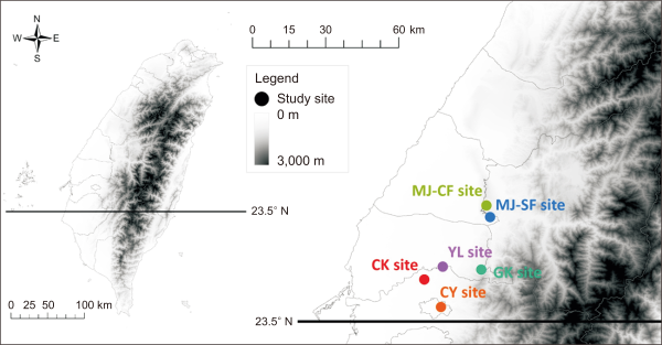
Fig. 2
Hierarchical cluster analysis of habitat groups. F, farmland cluster; B, bank cluster; CY-O, lychee orchard cluster at the Chia-Yi site; GK-O, lychee orchard cluster at the Gu-Keng site; T, tea garden cluster; CK, Chi-Ko site; YL, Yuin-Lin site; MJ, Min-Jian site; CF, conventional farming; SF, sustainable farming.
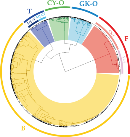
Fig. 3
Species–area curves for each microhabitat in the agricultural ecosystem for each season. F, farmland cluster; B, bank cluster; CY-O, lychee orchard cluster at the Chia-Yi site; GK-O, lychee orchard cluster at the Gu-Keng site; T, tea garden cluster.
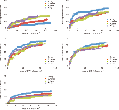
Table 1
Minimum quadrats for weed investigation in agricultural ecosystem
| Microhabitat cluster | Season | |||
|---|---|---|---|---|
|
|
||||
| Spring | Summer | Autumn | Winter | |
| F | 3.9 | 6.4 | 9.4 | 8.4 |
| B | 9.3 | 8.9 | 11.2 | 10.7 |
| CY-O | 16.2 | 15.0 | 18.0 | 13.2 |
| GK-O | 14.9 | 12.1 | 12.8 | 10.3 |
| T | 8.1 | 6.3 | 5.8 | 5.3 |
Table 2
Number of plant species and plant cover in the agricultural ecosystem of Taiwan during each season
| Season | P-value | ||||
|---|---|---|---|---|---|
|
|
|||||
| Spring | Summer | Autumn | Winter | ||
| (A) Species number | |||||
| F | 1.2±0.5c | 1.4±0.7c | 2.2±1.7a | 1.7±1.4b | *** |
| B | 4.1±2.4a | 3.4±2.2b | 3.4±1.8b | 2.4±1.5c | *** |
| CY-O | 5.9±2.2a | 5.1±2.0b | 5.6±2.1ab | 5.3±2.3ab | * |
| GK-O | 8.7±2.4a | 7.8±2.7b | 8.1±2.7ab | 6.7±1.9c | *** |
| T | 4.2±2.1a | 3.9±2.1a | 3.6±1.8a | 3.9±1.9a | ns |
| (B) Cover | |||||
| F | 71.5±25.3a | 34.1±35.3b | 69.8±35.9a | 17.0±27.8c | *** |
| B | 41.3±37.2b | 59.5±47.9a | 56.6±41.9a | 22.6±28.0c | *** |
| CY-O | 114.1±26.9ab | 103.2±30.3bc | 115.4±37.2a | 97.4±33.5a | *** |
| GK-O | 123.9±35.2ab | 131.6±36.5a | 131.3±33.0a | 116.9±39.5b | ** |
| T | 84.1±25.2ab | 90.5±19.8a | 84.9±20.8ab | 77.6±28.6b | ** |
F, farmland cluster; B, bank cluster; CY-O, lychee orchard cluster at the Chia-Yi site; GK-O, lychee orchard cluster at the Gu-Keng site; T, tea garden cluster.
*Indicates a significant difference among the seasons (one-way analysis of variance: *P<0.05, **P<0.01, ***P<0.001) and ns denotes no significant difference (one-way analysis of variance: P≥0.05). Numbers sharing letters indicate nonsignificant differences on the basis of a least significant difference test with a 5% significance level (mean±standard deviation).