Introduction
Since the three kinds of diversity, such as alpha diversity, beta diversity, and gamma diversity (α, β, and γ-diversity), were presented by Whittaker (1960; 1972), numerous ecological studies have been conducted using these concepts. According to Whittaker’s description, α-diversity is the local species diversity or richness in a single community and certain areas, whereas γ-diversity is the total species diversity or richness within a large number of sites on a regional scale. These two diversities are calculated by simple indices, such as the Shannon–Wiener index (Shannon, 1948) and Simpson’s index (Simpson, 1949), which are based on species richness and evenness (Thukral, 2017).
β-diversity is the spatial differentiation or variation in species composition among sites within a region (γ-diversity), which could also result from species replacement and loss within sites (Anderson et al., 2011; Baselga, 2010; Legendre et al., 2005). Since Whittaker (1960) proposed to compute β-diversity using the simple ratio between γ-diversity and mean value of α-diversity, several different estimates of β-diversity values using α and γ-diversity have been presented (Anderson et al., 2011; Koleff et al., 2003). However, the problem has been raised that β-diversity can only be derived after estimating the two diversity values (Ellison, 2010). To solve this problem, various methods for calculating β-diversity values without using the α and γ-diversity have been suggested, including a method using the total variance of the community data matrix (Anderson et al., 2006; Legendre & De Cáceres, 2013; Legendre et al., 2005; Pelissier & Couteron, 2007).
Legendre and De Cáceres (2013) and Legendre et al. (2005) introduced the calculation method for β-diversity as a single-number value, Var(Y) or BDTotal, based on the variance of the site-by-species community table (Y). With regard to beta diversity estimates based on the community table, β-diversity values could be calculated in two different ways: 1) the sum of squares of the species occurrence or abundance, and 2) dissimilarity matrix (Legendre & De Cáceres, 2013). The same value can be estimated by both methods and can be calculated without the numerical information from α- and γ-diversity. However, the β-diversity value could be differentiated depending on the dissimilarity coefficients. In order to provide guidance on the selection of dissimilarity coefficients for presence-absence (occurrence) and abundance (or biomass) data, 16 dissimilarity coefficients were compared according to the 14 properties. The local contribution to beta diversity (LCBD) value, the indices of which are derived from the calculation of the β-diversity estimate, was represented as “the degree of uniqueness of the sampling units in terms of community composition” (Legendre & De Cáceres, 2013).
In this study, we applied the β-diversity and LCBD concepts according to Legendre and De Cáceres (2013) to analyze fish community data, sampled from 13 sites along mid-low reaches of the Geum River in Korea. Specifically, we estimated β-diversity values depending on the two types of data, occurrence (with Jaccard and Sørensen dissimilarity coefficients) and abundance (with Hellinger distance) to represent the spatial variation of fish assemblages in the river. We also examined the degree of fish communities’ uniqueness on fish communities by calculation of LCBD values in each sites. Furthermore, in order to determine the ecological properties of the β-diversity results, we performed traditional correlation and multivariate analysis, non-metric multidimensional scaling (NMDS), on the fish data in company with the indices and values derived from the β-diversity concept.
Materials and Methods
Field sampling
To present the patterns of fish communities in the longitudinal river profile, 13 sampling sites were selected in the main channel of the Geum River (Fig. 1). The Geum River (397 km) is the third-longest river in Korea, flowing from the central area of the Korean Peninsula to the West Sea. The sample sites were located in the middle and lower reaches of the main channel of the river. The sampling site, S1, was at the upstream of the middle reach, located around 110 km upstream of the estuary of the West Sea (Fig. 1).
Fish assemblages were sampled monthly at each site from March to October 2019, a total of eight times. A kick net (5 mm mesh), cast net (mesh 7 mm; area πr2, 16.6 m2; r=2.3 m), and fyke net (mesh 5 mm, height 80, length 50 m) were used to collect the fish. Ten cast net deployments and kick nets for approximately 20 minutes were conducted for sampling in the shoreline area. Fyke nets were set perpendicular to the bank for 48 hours. All collected specimens were identified to the species level by following the keys according to Kim and Park (2002), based on the fish classification system of Nelson et al. (2016). Six environmental variables, including physicochemical and hydrological factors, were measured concurrently. Dissolved oxygen, electrical conductivity, hydrological variables, and substrata were measured in situ (YSI proplus® [YSI Inc., Yellow Springs, OH, USA] for water quality data). The substrate index (SI) was calculated based on the proportion of substrate composition in five particle size categories (Suren, 1996):
SI=0.07×% boulder+0.06×% cobble+0.05×% gravel+0.04×% sand +0.03×% mud/silt
Community indices and environmental variables at the sampling sites are summarized in Table 1. Sampling sites S1, S2, S3, and S4 are located in the middle reaches of the Geum River, with a high proportion of large substrates (boulders, cobbles, and pebbles) and velocity, and low water depth, whereas S11, S12, and S13 sites are in a typical lowland reach with small substrate particle size and deep water. The remaining sites, S5-S10, show intermediate environmental variables between the sites in the middle and lowland reaches (Table 1).
Data analysis
Single value estimates of β-diversity based on community dissimilarity matrix were applied to determine the variation of fish communities in the longitudinal river profile. The input data (Y), site-by-species community table, were used to calculate the β-diversity values, the total variance of Y (Var(Y)), and LCBD (Legendre & De Cáceres, 2013). Y consists of column vectors (presence-absence or abundance values of p species) and row vectors (n sampling sites). Indices i and j indicate the sampling unit (or sampling site) and fish species, respectively, and yij is the individual value of the presence-absence or abundance in community data matrix Y.
According to Legendre and De Cáceres (2013), estimation of β-diversity value (Var(Y)) consists of calculating the matrix of squared deviations from the column (species values) as follows:
where sij is the square of the difference between the yij value and (the mean value of the jth species). The sum of all the different values from all columns (SSTotal) is estimated as follows:
Var(Y), the total variance of the site-by-species community table, was calculated as follows:
BDTotal, which is the same value as Var(Y), can be considered as an estimate of the β-diversity values of the input data table (Legendre et al., 2005). The β-diversity values for the fish presence-absence data table were estimated based on two dissimilarity coefficients, the Jaccard similarity index, and the Sørensen index.
The calculation of Var(Y) using the above-mentioned equation, however, is not appropriate for the data table with raw values of species abundance, density, and biomass. The assessment of the dissimilarity between sites is based on the Euclidean distance. To estimate the β-diversity value (Var(Y)) based on the dissimilarity of abundance values, the Hellinger transformation was used to estimate the β-diversity values for site-by-species abundance input data tables (Legendre & De Cáceres, 2013).
The relative contribution of sampling site i to β-diversity values (LCBDi), is also computed as the sum of the sij values in each row i.
The monthly sampled community data at each site were pooled to estimate beta diversity and LCBDs. To reduce biases in beta diversity measures and multivariate analysis, rare species were excluded in the pooling process. Rarity weights (wi) estimation is performed as follows (Leroy et al., 2013):
where Qij is the number of occurrences of species i during eight sampling times, and Qjmin and Qjmax are the minimum and maximum occurrences in the species pool, respectively. rj is the chosen rarity cut-off point according to Gaston’s quartile definition (the first quartile of species occurrence, 25%) (Gaston, 1994). The maximum occurrence is defined as the highest occurrence among species.
To represent the relationships between the LCBD, biological indices, and environmental variables, a Pearson correlation analysis was conducted. In this regard, α-diversity values as a biological index were derived by measuring the Shannon diversity index (H'). NMDS ordination was also applied to determine the differences in longitudinal community patterns based on the similarities among species composition. All the analyses mentioned above were performed in the R environment.
Results
Community composition
A total of 42,659 fish individuals (excluding rare species) were collected and identified in three orders, nine families, and 36 species. The number of species and individuals at the sample sites ranged from 15 to 27 (mean: 21.5) and 1,063-9,078 (mean: 3,281.5), respectively. S10 showed the highest number of species and individuals, whereas the values were lowest in S1 (Table 1). Five species, Acheilognathus lanceolata, Pseudorasbora parva, Squalidus japonicus, Hemibarbus labeo, and Opsariichthys uncirostris, in the family Cyprinidae were widely distributed throughout all sampling sites in the middle and lowland reaches, whereas three species, Cyprinus carpio, Sarcocheilichthys variegatus, and Leiocassis ussuriensis, occurred in only one or two sampling sites.
Beta diversity estimation
We obtained the β-diversity values based on the total variance of the site-by-species data table containing the occurrence (presence-absence) and abundance information (Table 2). The β-diversity values (BDTotal or Var(Y)) and spatial variation of fish communities in the Geum River were calculated as 0.218 for the Jaccard dissimilarity index, 0.145 for the Sørensen index, and 0.268 for the Hellinger distance (Table 2). The total sum of squares (SSTotal) was also presented as 2.620, 1.738, and 3.211 for the Jaccard index, Sørensen index, and Hellinger distance, respectively.
We show the local contribution to beta diversity, LCBD, along the upstream (S1) to downstream (S13) in Fig. 2A. The LCBD of each site ranged from 0.060-0.114, 0.053-0.125, and 0.029-0.139 based on the Jaccard index, Sørensen index, and Hellinger distance. Higher LCBD values were estimated in the middle reaches of the Geum River, S1-S3, whereas lower values were observed in the lowland reach sites. The highest values of LCBD were computed in S1 for all the similarity indices. S7 shows the lowest values of LCBD for presence-absence data, whereas the lowest values of LCBD for abundance data are presented in S6. The number of species and α-diversity values at each site are presented in Fig. 2B. The number of species and H’ ranged from 15 to 27 and 2.146 to 2.623, respectively. Both values tend to be lower in the middle reaches of the Geum River, S1-S4. The highest values of H’ and the highest number of species were present in the sites on lowland reaches, S13 and S10 (Fig. 2).
Relationships between variables
Pearson correlation coefficients were obtained to show associations between the community and diversity indices (LCBDs and α-diversity) and environmental variables (Table 3). Strong positive correlations among the LCBD values for the three different similarity indices were detected. All LCBD values had strong negative correlations with the number of species (r=–0.861, –0.868, –0.795, respectively; P<0.01), whereas they were not significantly correlated with α-diversity and the number of individuals. The LCBD values based on occurrence data, LCBD(J) and LCBD(S), were negatively correlated with water temperature (r=–0.684 with P<0.01, –0.638 with P<0.05, respectively), whereas they were positively correlated with the SI (r=–0.611, –0.591, respectively; P<0.05). No significant correlation was observed between the environmental variables and LCBD(H).
Community ordination
In the NMDS ordination, the samples were distinguished based on differences in species composition in communities by Bray-Curtis dissimilarity (Fig. 3). The final stress value for the two dimensions was 0.063, which is acceptable for ecological and environmental data because it falls below 0.2. The sampling sites in the middle and lowland reach were separated along the NMDS axis 1. The fish communities at sampling sites were located in lowland reaches, S8-S13, and were aggregated on the right side of the map, whereas S1-S7 in the middle reach of the Geum River was widely distributed over the left side. Correlations between the NMDS axes and variables, including biological indices and environmental variables, were also presented to show the associations between fish communities and environments (Fig. 3). NMDS axes were significantly correlated with one biological index, LCBD values based on Jaccard similarity (r=0.49; P<0.05), and two environmental variables, water temperature (r=0.68; P<0.01) and depth (r=0.77; P<0.01).
Discussion
The application of β-diversity estimates based on community data tables and site-by-species occurrence and abundance effectively accounted for the spatial variation of fish communities in the Geum River. The β-diversity values were calculated as a single number without estimation of the α- and γ-diversity values. In addition, the β-diversity values of freshwater fish communities from two different rivers, the Geum River and the Doubs River in eastern France (Borcard et al., 2018; Legendre & De Cáceres, 2013), were compared. In the Geum River, three β-diversity values, including two values for occurrence data, 0.218 and 0.145, and a value for abundance data, 0.268, were presented according to the three different dissimilarity coefficients, Jaccard similarity index, Sørensen index and Hellinger distance, respectively (Table 2). The β-diversity values of fish communities in the Doubs River were 0.326, 0.267, and 0.503 for the same order of dissimilarity coefficients as aforementioned.
These results show that the β-diversity values for all dissimilarity coefficients were lower in the Geum River. It can be noted that spatial variations in fish assemblages were stronger in the Doubs River, although the total number of species in all fish assemblages was higher in the Geum River (36 species) than in the Doubs River (27 species). This result seems to be due to the higher connectivity of fish assemblages in the main channel of the Geum River or lack of fish community data, including rare species in tributary streams of the Geum River in mountainous areas. Further studies are required to determine the patterns of spatial variation of fish communities under various conditions, including the relationship between the main channel and tributaries, connectivity in the river channel, and disturbance intensity. For these approaches, more β-diversity analysis which related to the ecological properties in population or species level, such as species contribution to beta diversity (Legendre & De Cáceres, 2013), species replacement and species loss (Baselga, 2010), also should be considered in the future.
The present study also focused on LCBD values as an indicator of community uniqueness (Legendre & De Cáceres, 2013). NMDS ordination, a traditional multivariate analysis, and Pearson correlation were performed to examine the LCBD values as an indicator of community uniqueness in the Geum River (Fig. 3, Table 3). In the NMDS map, the distances between each pair of sites addressed the degree of differentiation of the communities due to the variability in species composition. Notably, the sites that were scattered widely over a long distance from other sites, S1 and S3, had higher LCBD values, whereas the sites with low LCBD values, S6 and 7, were concentrated around the center of the map at a close distance from other sites. The sites aggregated on the right side of the map showed relatively low LCBD (Figs. 2, 3). A significant correlation was also observed between the NMDS axes and LCBD for Jaccard dissimilarity coefficients (Fig. 3). Overall, the LCBD value was feasible for indicating the fish community uniqueness based on the dissimilarity of community composition in the Geum River. However, LCBD values were negatively correlated with the number of species (Table 3). Similar results were also reported in the fish community data from the Doubs River (Legendre & De Cáceres, 2013) and Cheonggye Stream (Kim et al., 2019). These results indicate that the uniqueness of fish communities is related to the small number of species and low α-diversity. However, this result seems unusual and counterintuitive. Further research is needed to reveal the relationships between LCBD and α-diversity indices, such as the number of species, species richness, and H’.
Considering LCBD values along the sampling sites in the Geum River, high LCBD values were obtained at sites S1 and S3, representing an environment with larger substrate size, higher water velocity, and lower water temperature (Fig. 2, Table 1). In addition, LCBD values were significantly correlated with two environmental variables: lower water temperature and larger substrate size (Table 3). These findings indicate that fish assemblages in the middle reaches of the Geum River contain several unique species or a small number of common species. Because of these properties, LCBD values have been suggested as an indicator of priority sites requiring conservation or restoration (Legendre & De Cáceres, 2013). However, more information regarding the relationships between LCBD values, α-diversity indices, and environmental variables is needed before using it as an indicator for conservation biology.
According to Legendre and De Cáceres (2013), the principle of the β-diversity estimate is similar to simple ordination methods for ecological community data, such as principal component analysis and canonical analysis, owing to the use of the total sum of squares. However, few studies have been conducted to reveal the relationship between β-diversity estimates and structural properties of the community, which is illustrated by species abundance distributions (SADs), and species-area relationships (SAR). Accordingly, further research is warranted regarding the relation of β-diversity estimates with SADs and SAR, in addition, and computational analysis for ecological data such as artificial neural network, random forests.
Figures and Table
Fig. 1
Map of the sampling sites in the Geum River in Korea. The study sites are indicated as yellow circles with site names.
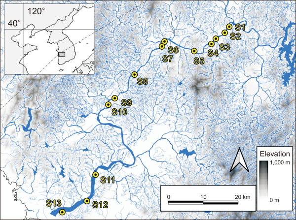
Fig. 2
Community indices at each sampling site, (A) estimated local contribution to beta diversity (LCBD) values based on three dissimilarity coefficients, Jaccard, Sørensen, and Hellinger distance (B) α-diversity (H’) and the number of species.
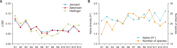
Fig. 3
Nonmetric multidimensional scaling (NMDS) ordination map based on fish communities with fitted vectors of community indices and environmental variables (red arrow: P<0.05, blue arrow: P>0.05). LCBD(J), local contribution to beta diversity based on Jaccard index; LCBD(S), local contribution to beta diversity based on Sørensen index; LCBD(H), local contribution to beta diversity based on Hellinger distance; H', α-diversity; No.sp., the number of species; No.indi., the number of individuals; W.temp., water temperature; DO, dissolved oxygen; Cond., electrical conductivity; Depth, water depth; Velocity, water velocity; SI, substrate index.
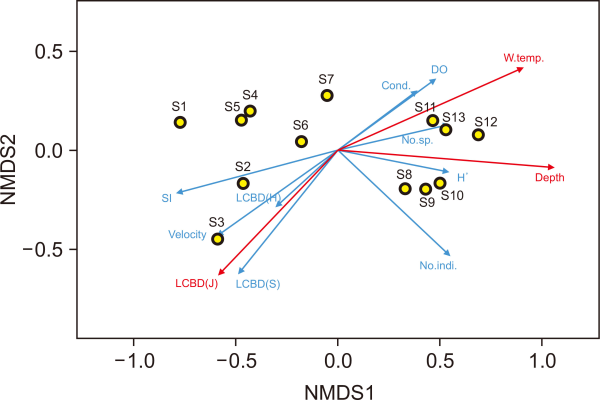
Table 1
Community indices and environmental variables at 13 sampling sites
| Sites | n | No. of individuals |
No. of species |
Water temperature (°C) |
Dissolved oxygen (mg/L) |
Conductivity (μs/cm) |
Depth (cm) | Velocity (cm/s) |
Substrate index |
|---|---|---|---|---|---|---|---|---|---|
| S1 | 8 | 1,063 | 15 | 18.8±3.9 | 11.3±2.2 | 236.7±36 | 62.5±19.1 | 32.8±18.3 | 3.69±0.52 |
| S2 | 8 | 1,707 | 21 | 19.1±4 | 10.7±1.3 | 284.5±43.4 | 111.3±18.9 | 15.9±10 | 1.62±0.08 |
| S3 | 8 | 1,319 | 17 | 20.3±4.4 | 11.6±2.7 | 292±48.5 | 83.8±19.2 | 82.8±25.4 | 4.28±0.47 |
| S4 | 8 | 2,027 | 22 | 20.9±4 | 12±2 | 336.3±52 | 88.8±15.5 | 83.2±23.8 | 4.05±0.69 |
| S5 | 8 | 1,756 | 20 | 20.2±4.3 | 10.8±2 | 320±39.1 | 213.8±37.4 | 19.3±9.8 | 3.15±0.78 |
| S6 | 8 | 1,870 | 25 | 21.3±5 | 11.8±2.1 | 285±82.5 | 153.8±57.1 | 14.2±4.2 | 2.74±0.63 |
| S7 | 8 | 4,849 | 25 | 20.6±4.8 | 11.9±1.4 | 292±81.3 | 153.8±73.7 | 13.9±3.3 | 2.59±0.82 |
| S8 | 8 | 4,104 | 23 | 20.8±5 | 12±2.7 | 288.6±89.7 | 196.3±123.2 | 11.2±2.6 | 2.34±0.7 |
| S9 | 8 | 7,253 | 23 | 20.9±5 | 11.5±3.1 | 311.5±57.1 | 393.8±195.7 | 10.8±1.4 | 2.59±0.51 |
| S10 | 8 | 9,078 | 27 | 21.2±5.3 | 11.5±2.8 | 301.1±53.1 | 416.3±114.9 | 13±1.9 | 2.28±0.74 |
| S11 | 8 | 2,501 | 21 | 22±5.9 | 11.8±2.4 | 300.6±74.6 | 261.3±70 | 28.4±32.6 | 1.8±0.7 |
| S12 | 8 | 3,073 | 19 | 21.8±6 | 12.9±3.6 | 306.1±68.6 | 373.8±143.5 | 8.7±3 | 2.36±1.25 |
| S13 | 8 | 2,059 | 21 | 21.6±5.9 | 11.3±2.3 | 324.3±79.5 | 457.5±147.9 | 5.7±2.4 | 1.88±1.25 |
Table 2
Total sum of squares and estimated beta diversity values of fish community data in the Geum River
| Dissimilarity coefficients | Presence-absence | Abundance | |
|---|---|---|---|
|
|
|
||
| Jaccard | Sørensen | Hellinger distance | |
| Total sum of squaresn (SSTotal) | 2.620 | 1.738 | 3.211 |
| Beta diversityn (Var(Y) or BDtotal) | 0.218 | 0.145 | 0.268 |
Table 3
Pearson correlations between biological indices and environmental variables
| Variable | Community and diversity indices | Environmental variables | ||||||||||
|---|---|---|---|---|---|---|---|---|---|---|---|---|
|
|
|
|||||||||||
| LCBD(S) | LCBD(H) | α-diversity (H') | No. of species | No. of individuals | Water temperature | DO | Conductivity | Depth | Velocity | SI | ||
| LCBD(J) | 0.995** | 0.749** | –0.481 | –0.861** | –0.471 | –0.684** | –0.196 | –0.501 | –0.494 | 0.477 | 0.611* | |
| LCBD(S) | 0.765** | –0.456 | –0.868** | –0.434 | –0.638* | –0.153 | –0.488 | –0.422 | 0.451 | 0.591* | ||
| LCBD(H) | 0.001 | –0.795** | –0.418 | –0.428 | –0.272 | –0.411 | –0.177 | 0.315 | 0.180 | |||
| α-diversity (H') | 0.148 | –0.004 | 0.403 | –0.087 | 0.108 | 0.410 | –0.317 | –0.578* | ||||
| No. of species | 0.689** | 0.462 | 0.110 | 0.350 | 0.355 | –0.387 | –0.435 | |||||
| No. of individuals | 0.316 | 0.138 | 0.173 | 0.590* | –0.383 | –0.307 | ||||||
| Water temperature | 0.592* | 0.606* | 0.651* | –0.185 | –0.348 | |||||||
| DO | 0.123 | 0.142 | 0.062 | 0.059 | ||||||||
| Conductivity | 0.461 | 0.113 | –0.081 | |||||||||
| Depth | –0.589* | –0.573* | ||||||||||
| Velocity | 0.805** | |||||||||||