Introduction
Ecosystem surveys are conducted for various purposes, such as for assessing environmental impacts before land development, predicting effects of such development, selecting protected areas, continuously monitoring whether currently protected areas are being properly maintained, or observing changes in the climate environment, among others (National Institute of Environmental Research (NIER), 2012; O et al., 2015). These surveys typically focus on understanding ecosystems within a survey area by examining nine taxonomic groups (mammals, birds, amphibians-reptiles, fish, insects, benthic macroinvertebrates, plants, vegetation, and topography), primarily identifying the fauna and flora. Results usually yield the number of species and individuals. Collected data are then appropriately analyzed according to the purpose and used for research or policy-making.
Traditional result of a biological survey is a species list. If it is possible to count individuals, various community analysis methods, including the selection of dominant species in the survey area, are also used. Conducting a complete census to determine how many species and individuals of organisms live in forests, rivers, lakes, etc., is almost impossible. Therefore, comparisons are often made by setting quantitative space or time for each survey site. For example, since most biological surveys tally the number of species and individuals, measures such as species diversity, species richness, dominance, evenness, and the number of common species are used to relatively evaluate or compare the biota of survey sites (Delang & Li, 2013; Han et al., 2016; Kang & Kang, 2018).
However, species diversity is a formula derived from Shannon’s information theory formula. It shows the highest entropy (H) value when all states are equal (Shannon, 1948). In other words, species diversity is the highest when every species in a surveyed species is distributed equally in individual numbers.
Shannon’s information theory formula,
where H is the entropy, n is the number of possible states of the message, p(xi) is the probability of a particular state (xi).
Species diversity formula, Shannon-Wiener Diversity Index
where H′ is the Shannon diversity index, S is the total number of species, pi is the number of individuals of the (i)th species divided by the total number of individuals.
Thus, the highest value of species diversity occurs when no dominant species exists, that is why it is used alongside other indicators such as species richness and dominance. Commonly, Margalef’s species richness index and Simpson’s dominance index are employed (Margalef, 1973; Simpson, 1949). Margalef’s index shows higher values when there is a greater number of species with fewer individuals, while Simpson’s index ranges from 0 to 1, indicating higher values when a few species (dominant and subdominant) are more abundant. These indices require the number of species and individuals for calculations. However, since they can be calculated regardless of the species type, they are not suitable for analyzing data observed over large areas or long periods. These indices are only valid for relative comparisons in small-scale surveys, both temporally and spatially. Additionally, because each index value represents different aspects, using various indices to describe the biota of a region can lead to confusion in understanding the ecosystem.
Subjective interpretation is essential even when biota data are quantified through index values. Ultimately, results of field survey evaluations can only be considered as insights and reflections based on the experience of long-practiced researchers.
It has been pointed out problems that can arise when quantifying biodiversity and collecting individual count information, emphasizing the importance of sampling efforts in the field and suggesting ways to avoid pitfalls that can occur when quantifying and comparing species richness (Gotelli & Colwell, 2001).
Additionally, research has pointed out limitations of previously used indices that represent biodiversity and species rarity with an aim to overcome them. New indices Sq and Eq have been proposed based on Tsallis entropy as alternatives to Shannon and Simpson’s indices (Mendes et al., 2008). However, these indices are mostly used for analyzing organisms within the same taxonomic group in a common area. They are not intended for comparative analysis across multiple taxonomic groups. Thus, their use is limited.
Ecosystems consist of various taxonomic groups of species interconnected through symbiosis, competition, predation, and other relationships. It has been challenging to express these connections numerically. To understand connections among species, scientific or statistical analysis is needed across taxonomic groups or regions. This has been difficult to explain with the indices described above. This research aimed to propose a new method of analysis focusing on connections between species rather than the traditional biodiversity index analysis based on species and individual counts. This new approach could help us understand ecosystem networks more effectively. In fact, network analysis methods for specific topics have already been widely used in other fields such as library and information science and social science.
Among them, co-occurrence frequency analysis can be used to identify connectivity and centrality in social and natural phenomena. It is often applied in text mining to refine keywords and analyze their meanings in many journal articles and research papers. This method has evolved as a tool for analyzing human social networks. It has recently become increasingly utilized in the field of ecology (Carrington et al., 2005; Lai et al., 2012).
In this research, the dataset from the ‘Ministry of Environment’s 4th National Natural Environment Survey (2014-2018)’ was used to analyze a wide range of data on survey areas and taxonomic groups, attempting to uncover inherent networks.
The ‘Ministry of Environment National Natural Environment Survey’ performed the first survey in 1986, followed by the second survey (1997-2005), the third survey (2006-2013), the fourth survey (2014-2018), and the fifth survey (2019-2023). Currently, the sixth survey is underway (National Institute of Ecology (NIE), 2023).
Dataset on the outcome of this survey provides vast information, offering nationwide location points and species-level information for nine taxonomic groups (mammals, birds, amphibians-reptiles, fish, insects, benthic macroinvertebrates, plants, vegetation, and topography).
There have been consistent studies using this dataset. However, most of them have focused on distribution patterns or predictions of important species within a single taxonomic group (endangered species, natural monuments, etc.) (Kim et al., 2012; Kwon et al., 2020a; Lee et al., 2017), methodologies for standardizing collected data, or information management systems using GIS (Kim et al., 2013; Kwon et al., 2020b).
Co-occurrence frequency analysis is often called semantic network analysis because it primarily produces five centrality indices (degree, weighted degree, closeness, betweenness, and eigenvector) to measure the importance of interrelationships. Values of these five centrality indices are used to analyze the meaning of the network (Bastian et al., 2009).
We utilized this dataset to perform a network analysis known as co-occurrence frequency analysis. We aimed to explore relationships inherent within it by generating frequencies of network connections between species identified during the same period (survey dates), within the same city or district, and at the same location (coordinates, location number). We analyzed both the degree and weighted degree.
Materials and Methods
Research area and taxa
Analysis data were derived from the 4th National Natural Environment Survey. The 4th National Natural Environment Survey was conducted over five years from 2014 to 2018. It covered nine taxa: topography, flora, phytosociology, mammals, Aves, amphibians and reptiles, insects, freshwater fishes, and benthic macroinvertebrates. Phytosociology was surveyed as its own evaluation unit, while the remaining eight taxa were surveyed based on a grid system of map sheets.
Map sheets divided Korea into 834 sections at a 1:25000 scale. Each map sheet was further divided into nine grids (referred to as NIE grid) arranged in a 3×3 format (E1, E2, ~, E9). Data for each taxonomic group were recorded at representative coordinates within the grid. In some cases, researchers recorded specific detailed coordinates. As the survey was conducted on one map sheet or one grid per day, collected species could be seen as a list of species that appeared simultaneously in the same space and time.
National Natural Environment Survey data were categorized and databased by taxonomic group, primarily consisting of metadata suitable for each group, including common and scientific names, higher classification systems, survey dates, map sheet and grid numbers, researcher names, coordinates, physical environment, and weather conditions. Table 1 shows items available for this study, with main data types needed for analysis being species names and spatial and temporal information, while metadata such as physical environment is not used (Table 1).
Among survey data, partial analysis was conducted for four taxonomic groups: herbaceous plants and woody plants for plants, butterflies for insects, and Passeriformes for birds. The remaining four groups, mammals, reptiles & amphibians, freshwater fishes, and benthonic macroinvertebrates, were analyzed across all species (Table 2). The reason for limiting taxonomic groups of plants, insects, and birds is as follows.
The total number of plant species is too large, making it difficult to find interspecies associations and necessitating the selection of certain groups. Herbaceous plants were assumed to be better than studying all species due to their shorter generations with many species that inhabit localized environments. Insects are the most diverse organisms. Expertise and survey ability among researchers may vary. Butterflies were chosen as the subject of analysis under the assumption that there would be the least variations among researchers. The reason for focusing on Passeriformes birds was that most of the survey map sheets were located in forests. In addition, most Passeriformes are forest-dwelling, thus excluding waterfowl and other birds.
Data analysis method
Co-occurrence frequency can be determined using items that distinguish time and space, with date, map sheet, grid, and coordinates being key items for identifying co-occurrence frequency. A list of species surveyed within a group can be obtained by grouping these items. In other words, grouping by map sheet – survey date – grid or survey date – map sheet – coordinates yields a list of species surveyed at the same place and time. Mammals and birds were grouped by date – map sheet – grid. The other six taxonomic groups were grouped by date – coordinates. This method was used to create detailed groups. A compilation of analyzed data is shown in Table 2.
Data surveyed over five years were used for data analysis (Table 2). Herbaceous plants comprising 494 species from 456 map sheets were divided into 8213 detailed groups. Woody plants comprising 256 species from 453 map sheets were divided into 7020 detailed groups. Mammals consisting of 54 species from 632 map sheets were divided into 4030 detailed groups. Passeriformes comprising 132 species from 518 map sheets were divided into 2891 detailed groups. Butterflies consisting of 161 species from 408 map sheets were divided into 1472 detailed groups. Amphibians and reptiles comprising 42 species from 424 map sheets were divided into 3842 detailed groups. Freshwater fishes consisting of 143 species from 411 map sheets were divided into 2861 detailed groups. Benthic macroinvertebrates consisting of 93 species from 350 map sheets were divided into 1741 detailed groups. All of these were used for analysis. Map sheets surveyed annually by the taxonomic group are as shown in Fig. 1.
Furthermore, the list of species thus obtained was expressed as a combination set to calculate the co-occurrence frequency. When the set of species confirmed at each survey point (or NIE grid) Pi is denoted as Spi, the list of species can be expressed mathematically for the combination set as follows:
To explain the above formula, it can be described as follows. For example, let’s define the set of species found at each survey point P1, P2, …, Pi as Sp1, Sp2, …, Spi, respectively. If the species found at P1 are (a, b, c, d) and the species found at P2 are (b, d, e), then we can express Sp1 = {a, b, c, d}, Sp2 = {b, d, e}. Elements (species) of Sp1 and Sp2 are used as nodes. This can be presented as a set of subsets consisting of two elements from the P1 point as follows:
This combination set can again be expressed as an edge set with
Therefore, it can be generalized as a graph of the set NWG (network graph) with nodes S and edges E, which can be mathematically expressed as follows:
Elements of Epi are ordered pairs, which can be displayed in the typical graph notation G = (V, E). With this, we produced network graph data dealt with in set theory.
Due to a large number of groups and species, the creation of such combination sets was carried out using development tools for Python 3.x such as Spyder 5.1.x and Jupyter Notebook 6.4.x. Analysis modules for the generated network graphs utilized libraries such as Numpy, Pandas, and Networkx.
Results
Meaning of the index value and significance of the regression fit line
An analysis of the co-occurrence frequency for eight taxonomic groups was performed. Results are shown in Table 3.
In the study, 94 species of herbaceous plants generated 34,648 edges (degrees), 256 species of woody plants generated 11,336 edges, 54 species of mammals generated 634 edges, 132 species of Passeriformes generated 6,183 edges, 161 species of butterflies generated 6,662 edges, 42 species of amphibians & reptiles generated 555 edges, 143 species of freshwater fish generated 3,728 edges, and 93 species of benthonic macro invertebrates generated 1,468 edges. The above edge value is that connects events in which one species appears simultaneously with other species only once without accumulating them. The total species degree index for all species showed a correlation coefficient (R2) value of 0.968. However, this result is not particularly meaningful because it is a natural outcome of the fact that the total degree value increases as the total number of species increases. Nevertheless, no correlation was shown for the total number of species vs. weighted degree (R2 = 0.076) or the degree vs. weighted degree (R2 = 0.054).
Assuming that certain species coexist uniformly in the same space at the same time, if these species were observed simultaneously, the number of species, the degree of connectivity, and the cumulative frequency would be proportional. Therefore, even if the taxa are different, they can exhibit a similar pattern. Results showed that species did not appear to be distributed evenly. Therefore, it was difficult to find any significance in the total number of species, degree value, and weighted degree value from the co-occurrence frequency. However, the linear regression slope based on degree value was aggregated to be around 0.8 and the average value of the clustering coefficient also appeared to be around 0.8 (Table 3).
Fig. 2 shows the degree value of co-occurrence frequency for each of the eight taxonomic groups. The horizontal axis arranges species with the lowest degree value on the left and the highest on the right. The vertical axis represents the degree value as a scatter plot. The X-axis represents the sequence number of the species. The Y-axis represents the number of species most connected to the corresponding sequence number. For example, the horizontal axis for 494 herbaceous species would be 494. However, the vertical axis would not exceed 493. For amphibians and reptiles, the horizontal axis would be 42 species and the vertical axis would not exceed 41 species. Despite not being standardized to 100 or 1, most taxonomic groups obtained an almost linear scatter plot. The coefficient of determination was higher than 0.9 for all taxonomic groups. Excluding sparrows and amphibians & reptiles, it was above 0.97, which was almost linear. The slope was around 0.8.
Fig. 3 shows weighted degree (cumulative connectivity) of co-occurrence frequency for each of the eight taxonomic groups. The horizontal axis arranges the species with the lowest cumulative connectivity (weighted degree) on the left and the highest on the right, similar to Fig. 2. The vertical axis represents the cumulative connectivity (weighted degree) value as a scatter plot. The horizontal axis cannot exceed the number of species, but the vertical axis has different upper limits depending on the number of co-occurrence frequencies. These graphs obtained a very high nonlinear regression trend line as an exponential curve, with the coefficient of determination R2 exceeding 0.95 for all taxonomic groups. These two graphs indicate the presence of species distributed regionally and those distributed widely.
This is the type seen as having random connections, a typical type of the W-S model (Watts & Strogatz, 1998). The W-S model is mostly found in natural states. Although it may seem like an ordinary phenomenon (result), it has significant meaning. It allows for measuring the past or current state of commonly seen general and rare species. The weighted degree value increases exponentially, which appears to be in the form of the ERGM (Exponential random graph model). It can be analyzed using analytical techniques developed in sociology (Lusher et al., 2013). If more preliminary research and analysis are conducted by further subdividing taxonomic groups or grouping, there is a possibility of discovering the B-A model, which has connectivity in the form of a power law (Barabási & Albert, 1999).
To explain Fig. 2 again, a slope of 0.8 means that the next species in the sequence of connectivity has 0.8 more species connected than the previous species. Since it is almost linear, there is no specific group of species. These taxonomic groups include orders such as the Passeriformes, two classes (amphibians and reptiles), phylum-level groups such as benthic macroinvertebrates, and mixed cases of various orders and families such as herbaceous and woody plants. Mammals are a single class-level group. Despite being artificially grouped, they show similar results. The average value of the clustering coefficient in Table 3 is 0.8, which means that the number of interconnected species is about 80% of the total species. This did not seem to be a coincidence because all eight taxonomic groups showed similar results. This 80% ratio is a common phenomenon in human society.
From these results, it can be inferred that spatiotemporal distribution patterns of species are not uniform, with species ranging from those distributed regionally to those distributed widely. There seems to be some rules regardless of the taxonomic group. To make it clearer what these few rules are, much additional research will need to be conducted.
Meaning of network graphs
Fig. 4 is a simple connectivity graph that explains this random connection state. For the eight taxonomic groups, species with high degree connectivity, i.e., those distributed widely, were placed at the top and species with low connectivity, i.e., those distributed locally, were divided into five levels and placed at the bottom. It could be seen that each taxonomic group had different proportions of species at each level. Herbaceous species had more locally distributed species than widely distributed ones. Conversely, amphibian & reptile species had fewer locally distributed species. Although they are both plants, woody species appeared to have a similar proportion of species at each level, unlike herbaceous species. Passeriformes species seemed to have a higher proportion of locally distributed species. Freshwater fish and benthonic macroinvertebrates had relatively fewer widely distributed species at the top compared to other taxonomic groups. The other four levels appeared similar. Mammals seemed to be divided into two groups at the very bottom, which were locally distributed species, likely because the researchers who surveyed bats and rodents were differentiated. The total degree and weighted degree values in Table 3 were similar to species diversity and richness. While combining all into one number can yield an intuitive answer, it does not reflect various meanings.
Thus, degree (connectivity) can be expressed in graphs not only in the form of Fig. 4, but also in various other graphs. It can also be implemented in 3D for intuitive visualization and exploration. It is possible to represent it as a visualization graph that intuitively shows the position of species with high centrality or high connectivity (Bastian et al., 2009). It is possible to express levels according to each index in various ways. Since many visualization tools have already been developed, analysis can be done through interactive dynamic materials and static image files.
Discussion
Like the first law of geography, everything is connected to everything else and closer things are more related than those farther away (Tobler, 1970). This method of connecting species that are close in time and space can produce results that are relatively easy to implement and carry a lot of meaning.
In our country, most of the biota survey data are investigated and compiled in the form of a national environmental survey. This means that co-occurrence frequency analysis is possible for almost all biota data. Moreover, most of these data are publicly available or can be obtained through a few procedures. Although this paper analyzed the taxonomic group, data surveyed at the same place and time were not related to the taxonomic group.
For example, repeated surveys over a certain period of insects, herbaceous plants, benthic animals, and plankton occurring in a small pond can make the food web network of that ecosystem. If the time unit is morning, afternoon, or 24 hours and the spatial unit is refined to coordinates, the resolution of co-occurrence frequency will be higher. By grouping certain sets of species into specific place and time (period) for analysis, it seems possible to find out interactions between species under certain conditions. It is also possible to analyze survey points or regions as units of groups of biological species. It is about finding out the connectivity of places where certain species occur. Projecting the dispersion of alien species onto a spatial map is also possible.
As mentioned in the introduction, analysis of biota survey data has been limited to short-term, small-scale survey areas compared to the amount of survey data, so it has relied mainly on subjective consideration of experts. It includes the tally of species and individual counts, as well as diversity, richness, and dominance. In South Korea, the environmental impact assessment system’s natural ecological environment sector’s flora and fauna reports are utilized the most by the analysis mentioned above. Reports are also written to lower the grade of our country’s ecological natural map of the development target area in the pre-development planning stage, similar to those of the environmental impact assessment. Similar to environmental impact assessment, ecological naturalness grades are mostly readjusted (Jung et al., 2017; Kim et al., 2023; Oh et al., 2023). If used properly, we believe that this analytical method can complement conventionally entrenched methods of analyzing diversity, richness, and dominance.
Since there are no restrictions on time or space, data surveyed in a small area over a short period and those accumulated over a long period on a national scale can be analyzed through proper grouping. Therefore, this analysis seems to overcome limitations of biological species data. The fact that co-occurrence frequency analysis can measure how many species one species is associated with and how frequently each species is associated with each other will be of great help in understanding ecosystems that seem too complex to know. Such connectivity data and graphs generated by the co-occurrence frequency analysis of biota are thought to provide a wealth of data and insights to researchers and those who observe, manage, and lives in ecosystems. It is hoped that this method will analyze a lot of ecological data that have been accumulated or are accumulating.
Acknowledgment
This study was conducted based on results of the 4th National Ecosystem Survey of the National Institute of Ecology (NIE). This work was also supported by a grant (NIE-A-2024-01) from the 6th National Ecosystem Survey of the National Institute of Ecology (NIE) funded by the Ministry of Environment (MOE), Republic of Korea.
Author Contributions
YK analyzed data and wrote the original draft. JB analyzed the data, reviewed the draft, and participated in writing the introduction. SJ and JH participated in extracting and processing the data needed for analysis. All authors have read and approved the final manuscript.
Figures and Tables
Fig. 1
Index map used in the analysis of each taxon. A. Index map sheet showing the entire 1:25,000 scale map. B to H, Survey index map of each taxonomic group surveyed separately over five years (2014-2018).
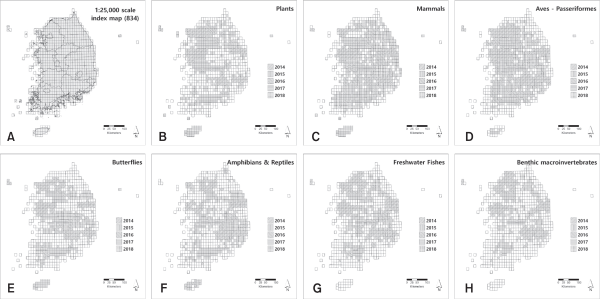
Fig. 2
Degree scatter plot of co-occurrence frequency for eight taxa. The horizontal axis is the number of species listed sequentially from the least degree species to the most degree species. The vertical axis is a scatter plot of species degree.
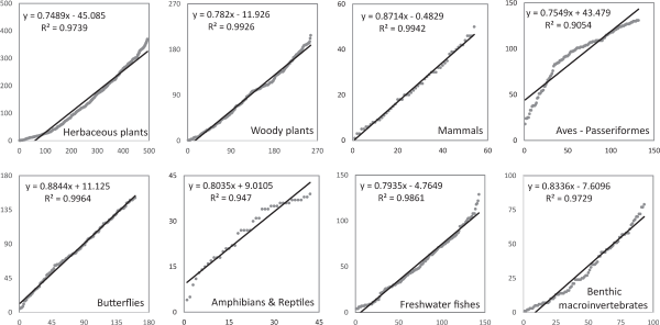
Fig. 3
Weighted degree scatter plot of co-occurrence frequency for eight taxa. The horizontal axis is the number of species listed sequentially from the least weighted degree species to the most weighted degree species. The vertical axis is a scatter plot of species weighted degree.
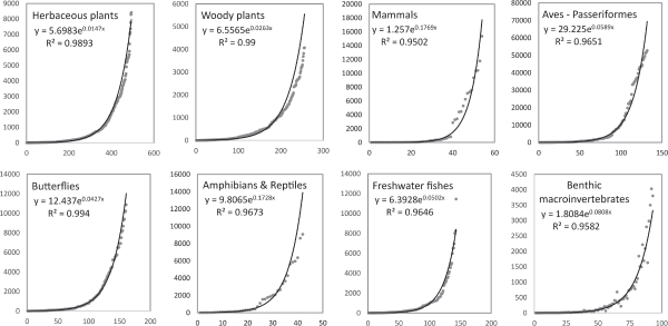
Fig. 4
Network graphs for each taxon drawn in five dimensions (distinctions). Although the number of nodes (species) and the number of edges are different for each taxon, the wide distribution (common species) and locally distributed species appear similar in all graphs.
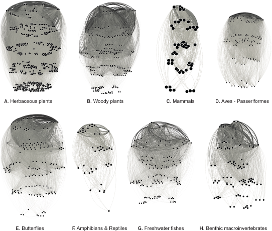
Table 1
Main components of survey data used in the analysis
| Component | Principal contents | Available |
|---|---|---|
| Date | The date is recorded as year, month and day. Date information is a good form of data because it allows time and space to be distinguished by changing the date even if repeated surveys are conducted at the same site. | used |
| 1/25000 index map and nine grids | The 1:25000 index map and grid are basic data for classifying spatial data. They were used to classify groups. | used |
| Name | Because local and scientific names only use the list published in the guidelines to avoid synonymy, species duplication does not occur. Therefore, it was used as a node without any special processing. | used |
| Taxa | Only some subtaxa were used for plants, insects, and birds with a large number of species. For plants, data from herbaceous and woody species were used. For insects, only butterflies were analyzed. For birds, only Passeriformes were analyzed. For other taxa mammals, amphibians & reptiles, fresh water fishes, and benthic macroinvertebrates, all recorded species were used in the analysis. | used |
| Coordinates | For plants, butterflies, fish, and benthic macroinvertebrates, coordinates were used for grouping. For mammals and passerines, an index map and NIE grids were used for grouping. | used |
| Meta data | Metadata such as surveyor, higher taxonomic group, and physical environment of the survey site were not used because it was difficult to process them into homogeneous data for grouping by time and space. | not used |
Table 2
Groups and species of data used in the analysis
| Taxa | No. of species | Survey year | No. of 1/25000 map | No. of group (set) |
|---|---|---|---|---|
| Herbaceous plants | 494 | 5 | 456 | 8,213 |
| Woody plants | 256 | 5 | 453 | 7,020 |
| Mammals | 54 | 5 | 632 | 4,030 |
| Passeriformes | 132 | 5 | 518 | 2,891 |
| Butterflies | 161 | 5 | 408 | 1,472 |
| Reptiles & Amphibians | 42 | 5 | 424 | 3,842 |
| Freshwater Fishes | 143 | 5 | 411 | 2,861 |
| Benthic macro invertebrates | 93 | 5 | 350 | 1,741 |
Table 3
Nodes, edges, and other indices of data used in the analysis
| Taxa | No. of node | No. of degree (edges) | No. of cumulated degree (edges) | Slope of linear regression on degree index | Avg. of cluster coefficient |
|---|---|---|---|---|---|
| Herbaceous plants | 494 | 34,648 | 247,934 | 0.749 | 0.798 |
| Woody plants | 256 | 11,336 | 88,423 | 0.782 | 0.783 |
| Mammals | 54 | 634 | 57,602 | 0.871 | 0.826 |
| Passeriformes | 132 | 6,183 | 605,519 | 0.804 | 0.883 |
| Butterflies | 161 | 6,662 | 138,543 | 0.884 | 0.841 |
| Reptiles & Amphibians | 42 | 555 | 37,017 | 0.755 | 0.858 |
| Freshwater Fishes | 143 | 3,728 | 80,144 | 0.794 | 0.807 |
| Benthic macro invertebrates | 93 | 1,468 | 22,477 | 0.834 | 0.827 |