JOURNAL OF INFORMATION SCIENCE THEORY AND PRACTICE
- P-ISSN2287-9099
- E-ISSN2287-4577
- SCOPUS, KCI
 ISSN : 2287-9099
Characterization of New Two Parametric Generalized Useful Information Measure

M. A. K. Baig (Post Graduate Department of Statistics University of Kashmir)

Abstract
In this paper we define a two parametric new generalized useful average code-word length <math xmlns="http://www.w3.org/1998/Math/MathML"> <msubsup> <mtext>L</mtext> <mtext>α</mtext> <mtext>β</mtext> </msubsup> </math>(P;U) and its relationship with two parametric new generalized useful information measure <math xmlns="http://www.w3.org/1998/Math/MathML"> <msubsup> <mtext>H</mtext> <mtext>α</mtext> <mtext>β</mtext> </msubsup> </math>(P;U) has been discussed. The lower and upper bound of <math xmlns="http://www.w3.org/1998/Math/MathML"> <msubsup> <mtext>L</mtext> <mtext>α</mtext> <mtext>β</mtext> </msubsup> </math>(P;U), in terms of <math xmlns="http://www.w3.org/1998/Math/MathML"> <msubsup> <mtext>H</mtext> <mtext>α</mtext> <mtext>β</mtext> </msubsup> </math>(P;U) are derived for a discrete noiseless channel. The measures defined in this communication are not only new but some well known measures are the particular cases of our proposed measures that already exist in the literature of useful information theory. The noiseless coding theorems for discrete channel proved in this paper are verified by considering Huffman and Shannon-Fano coding schemes on taking empirical data. Also we study the monotonic behavior of <math xmlns="http://www.w3.org/1998/Math/MathML"> <msubsup> <mtext>H</mtext> <mtext>α</mtext> <mtext>β</mtext> </msubsup> </math>(P;U) with respect to parameters α and β. The important properties of <math xmlns="http://www.w3.org/1998/Math/MathML"> <msubsup> <mtext>H</mtext> <mtext>α</mtext> <mtext>β</mtext> </msubsup> </math>(P;U) have also been studied.
- keywords
- Shannon's entropy, codeword length, useful information measure, Kraft inequality, Holder's inequality, Huffman codes, Shannon-Fano codes, Noiseless coding theorem
1. INTRODUCTION / LITERATURE REVIEW
The growth of telecommunication in the early twentieth century led several researchers to study the information control of signals, the seminal work of Shannon [17], based on papers by Nyquists [14], [15] and Hartley [7] rationalized these early efforts into a coherent mathematical theory of communication and initiated the area of research now known as information theory. The central paradigm of classical information theory is the engineering problem of the transmission of information over a noisy channel. The most fundamental results of this theory are Shannon's source coding theorem which establishes that on average the number of bits needed to represent the result of an uncertain event is given by its entropy; and Shannon's noisy-channel coding theorem which states that reliable communication is possible over noisy channels provided that the rate of communication is below a certain threshold called the channel capacity. Information theory is a broad and deep mathematical theory with equally broad and deep applications, amongst which is the vital field of coding theory. Information theory is a new branch of probability and statistics with extensive potential application to communication system. The term information theory does not possess a unique definition. Broadly speaking, information theory deals with the study of problems concerning any system. This includes information processing, information storage and decision making. In a narrow sense, information theory studies all theoretical problems connected with the transmission of information over communication channels. This includes the study of uncertainty (information) measure and various practical and economical methods of coding information for transmission.
It is a well-known fact that information measures are important for practical applications of information processing. For measuring information, a general approach is provided in a statistical framework based on information entropy introduced by Shannon (1948) as a measure of information. The Shannon entropy satisfies some desirable axiomatic requirements and also it can be assigned operational significance in important practical problems, for instance in coding and telecommunication. In coding theory, usually we come across the problem of efficient coding of messages to be sent over a noiseless channel where our concern is to maximize the number of messages that can be sent through a channel in a given time. Therefore, we find the minimum value of a mean codeword length subject to a given constraint on codeword lengths. As the codeword lengths are integers, the minimum value lies between two bounds, so a noiseless coding theorem seeks to find these bounds which are in terms of some measure of entropy for a given mean and a given constraint. Shannon (1948) found the lower bounds for the arithmetic mean by using his own entropy. Campbell (1965) defined his own exponentiated mean and by applying Kraft’s (1949) inequality, found lower bounds for his mean in terms of Renyi’s (1961) measure of entropy. Longo (1976) developed lower bound for useful mean codeword length in terms of weighted entropy introduced by Belis and Guiasu (1968). Guiasu and Picard (1971) proved a noiseless coding theorem by obtaining lower bounds for another useful mean code-word length. Gurdial and Pessoa (1977) extended the theorem by finding lower bounds for useful mean codeword length of order α; also various authors like Jain and Tuteja (1989), Taneja et al (1985), Hooda and Bhaker (1997), and Khan et al (2005) have studied generalized coding theorems by considering different generalized ‘useful’ information measures under the condition of unique decipherability.
In this paper we define a new two parametric generalized useful average code-word length <math xmlns="http://www.w3.org/1998/Math/MathML"> <msubsup> <mtext>L</mtext> <mtext>α</mtext> <mtext>β</mtext> </msubsup> </math> (P;U) and discuss its relationship with new two parametric generalized useful information measure <math xmlns="http://www.w3.org/1998/Math/MathML"> <msubsup> <mtext>H</mtext> <mtext>α</mtext> <mtext>β</mtext> </msubsup> </math>(P;U). The lower and upper bound of, <math xmlns="http://www.w3.org/1998/Math/MathML"> <msubsup> <mtext>L</mtext> <mtext>α</mtext> <mtext>β</mtext> </msubsup> </math> (P;U) in terms of <math xmlns="http://www.w3.org/1998/Math/MathML"> <msubsup> <mtext>H</mtext> <mtext>α</mtext> <mtext>β</mtext> </msubsup> </math>(P;U) are derived for a discrete noiseless channel in Section 3. The measures defined in this communication are not only new but also generalizations of certain well known measures in the literature of useful information theory. In Section 4, the noiseless coding theorems for discrete channels proved in this paper are verified by considering Huffman and Shannon-Fano coding schemes using empirical data. In Section 5, we study the monotonic behavior of <math xmlns="http://www.w3.org/1998/Math/MathML"> <msubsup> <mtext>H</mtext> <mtext>α</mtext> <mtext>β</mtext> </msubsup> </math>(P;U) with respect to parameters α and β. Several other properties of <math xmlns="http://www.w3.org/1998/Math/MathML"> <msubsup> <mtext>H</mtext> <mtext>α</mtext> <mtext>β</mtext> </msubsup> </math>(P;U) are studied in Section 6.
2. BASIC CONCEPTS
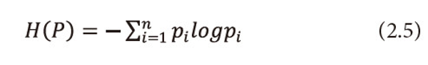
iLet X be a finite discrete random variable or finite source taking values x1,x2,…,xn with respective probabilities P = (p1,p2,…,pn),pi ≥ 0 ⩝ i = 1,2,...,n and <math xmlns="http://www.w3.org/1998/Math/MathML"> <msubsup> <mtext>Σ</mtext> <mrow> <mi>i</mi> <mo>=</mo> <mn>1</mn> </mrow> <mi>n</mi> </msubsup> </math>Pi=1. Shannon [1948] gives the following measure of information and call it entropy.
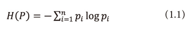
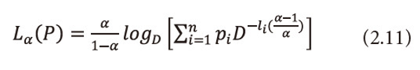
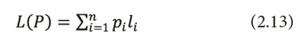
The measure (1.1) serves as a suitable measure of entropy. Let p1,p2,p3,…,pn be the probabilities of n codewords to be transmitted and let their lengths l1,l2,…,ln satisfy Kraft (1949) inequality,
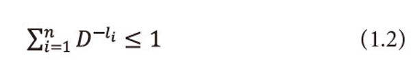
For uniquely decipherable codes, Shannon (1948) showed that for all codes satisfying (1.2), the lower bound of the mean codeword length,
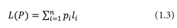
lies between H(P) and H(P)+1, where D is the size of code alphabet.
Shannon’s entropy (1.1) is indeed a measure of uncertainty and is treated as information supplied by a probabilistic experiment. This formula gives us the measure of information as a function of the probabilities only in which various events occur without considering the effectiveness or importance of the events. Belis and Guiasu (1968) remarked that a source is not completely specified by the probability distribution P over the source alphabet X in the absence of quality character. They enriched the usual description of the information source (i.e., a finite source alphabet and finite probability distribution) by introducing an additional parameter measuring the utility associated with an event according to their importance or utilities in view of the experimenter.
Let U = u1,u2,…,un be the set of positive real numbers, where ui is the utility or importance of outcome xi. The utility, in general, is independent of <math xmlns="http://www.w3.org/1998/Math/MathML"><mtext>Ρ</mtext></math>i, i.e., the probability of encoding of source symbol xi. The information source is thus given by
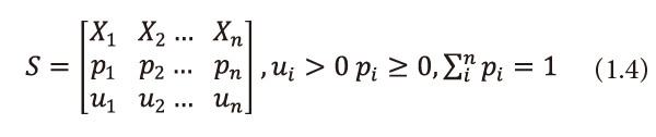
We call (1.4) a Utility Information Scheme. Belis and Guiasu (1968) introduced the following quantitative - qualitative measure of information for this scheme.
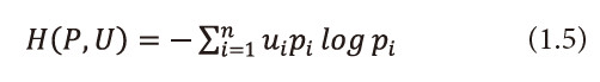
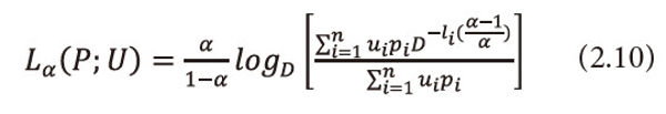
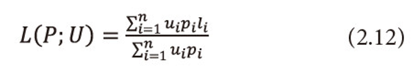
and call it as ‘useful’ entropy. The measure (1.5) can be taken as satisfactory measure for the average quantity of ‘valuable’ or ‘useful’ information provided by the information source (1.4). Guiasu and Picard (1971) considered the problem of encoding the letter output by the source (1.4) by means of a single letter prefix code whose codeword’s c1,c2,…,cn have lengths l1,l2,…,ln respectively and satisfy the Kraft’s inequality (1.2), they introduced the following quantity
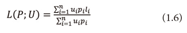
and call it as ‘useful’ mean length of the code. Further, they derived a lower bound for (1.6). However, Longo (1976) interpreted (1.6) as the average transmission cost of the letters xi with probabilities Pi and utility and gave some practical interpretations of this length; bounds for the cost function (1.6) in terms of (1.5) are derived by him.
3. NOISELESS CODING THEOREMS FOR ‘USEFUL’ CODES
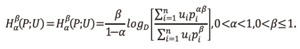
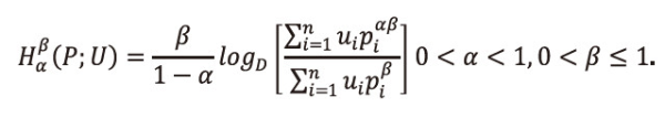
Define a two parametric new generalized useful information measure for the incomplete power distribution as:
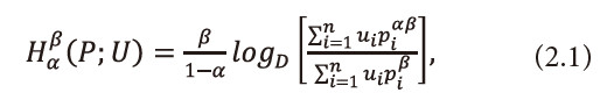
Where 0<α<1,0<β≤1,pi≥0 =1,2,…,n ,<math xmlns="http://www.w3.org/1998/Math/MathML"> <msubsup> <mtext>Σ</mtext> <mrow> <mi>i</mi> <mo>=</mo> <mn>1</mn> </mrow> <mi>n</mi> </msubsup> <mtext>Ρi</mtext> <mo>≤</mo> <mn>1</mn> </math>
Remarks for (2.1)
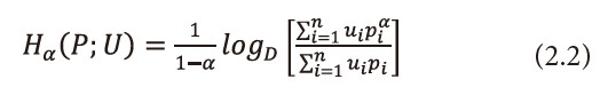
Ⅰ. When β=1, (2.1) reduces to ‘useful’ information measure studied by Taneja, Hooda, and Tuteja (1985), i.e.,
Ⅱ. When β=1, =1, =1,2,…,n, i.e., when the utility aspect is ignored and <math xmlns="http://www.w3.org/1998/Math/MathML"> <msubsup> <mtext>Σ</mtext> <mrow> <mi>i</mi> <mo>=</mo> <mn>1</mn> </mrow> <mi>n</mi> </msubsup> <mtext>Ρi</mtext> <mo>≤</mo> <mn>1</mn> </math>, (2.1) reduces to Reyni’s (1961) entropy, i.e.,
Ⅲ. When β=1 and α→1, (2.1) reduces to ‘useful’ information measure for the incomplete distribution due to Bhakar and Hooda (1993), i.e.,

Ⅳ. When β=1, =1, =1,2,…,n, i.e., when the utility aspect is ignored, <math xmlns="http://www.w3.org/1998/Math/MathML"> <msubsup> <mtext>Σ</mtext> <mrow> <mi>i</mi> <mo>=</mo> <mn>1</mn> </mrow> <mi>n</mi> </msubsup> <mtext>Ρi</mtext> <mo>≤</mo> <mn>1</mn> </math> and α→1, the measure (2.1) reduces Shannon’s (1948) entropy, i.e.,
When β=1, =1, =1,2,…,n, i.e., when the utility aspect is ignored, <math xmlns="http://www.w3.org/1998/Math/MathML"> <msubsup> <mtext>Σ</mtext> <mrow> <mi>i</mi> <mo>=</mo> <mn>1</mn> </mrow> <mi>n</mi> </msubsup> <mtext>Ρi</mtext> <mo>≤</mo> <mn>1</mn> </math>, α→1, and 1,2,…,n, the measure (2.1) reduces to maximum entropy, i.e.,

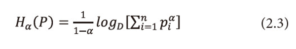
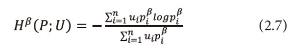
Ⅵ. When α→1, the measure (2.1) reduces to useful information measure for the incomplete power distribution pβ due to Sharma, Man Mohan, and Mitter (1978), i.e.,
Ⅶ. When α→1, =1, =1,2,…,n, i.e., when the utility aspect is ignored, (2.1) reduces to a measure of incomplete power probability distribution due to Mitter and Mathur (1972), i.e.,

Further, we define a two parametric new generalized useful average code-word length corresponding to (2.1) and is given by
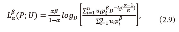
Where 0<α<1,0<β≤1,pi≥0 <math xmlns="http://www.w3.org/1998/Math/MathML"> <mo>∀</mo> <mi>i</mi> </math>=1,2,…,n, <math xmlns="http://www.w3.org/1998/Math/MathML"> <msubsup> <mtext>Σ</mtext> <mrow> <mi>i</mi> <mo>=</mo> <mn>1</mn> </mrow> <mi>n</mi> </msubsup> <mtext>Ρi</mtext> <mo>≤</mo> <mn>1</mn> </math> and D is the size of code alphabet.
Remarks for (2.9)
Ⅰ. When β=1, (2.9) reduces to ‘useful’ average codeword length due to Taneja, Hooda, and Tuteja (1985), i.e.,
Ⅱ. When β=1, ui=1, <math xmlns="http://www.w3.org/1998/Math/MathML"> <mo>∀</mo> <mi>i</mi> </math>=1,2,…,n, i.e., when the utility aspect is ignored and <math xmlns="http://www.w3.org/1998/Math/MathML"> <msubsup> <mtext>Σ</mtext> <mrow> <mi>i</mi> <mo>=</mo> <mn>1</mn> </mrow> <mi>n</mi> </msubsup> <mtext>Ρi</mtext> <mo>≤</mo> <mn>1</mn> </math>, (2.9) reduces to exponentiated mean codeword length due to Campbell (1965) entropy, i.e.,
Ⅲ. When β=1 and α→1, (2.9) reduces to ‘useful’ codeword length due to Guiasu and Picard (1971), i.e.,
Ⅳ. When β=1, ui=1, <math xmlns="http://www.w3.org/1998/Math/MathML"> <mo>∀</mo> <mi>i</mi> </math> =1,2,…,n, i.e., when the utility aspect is ignored, <math xmlns="http://www.w3.org/1998/Math/MathML"> <msubsup> <mtext>Σ</mtext> <mrow> <mi>i</mi> <mo>=</mo> <mn>1</mn> </mrow> <mi>n</mi> </msubsup> <mtext>Ρi</mtext> <mo>≤</mo> <mn>1</mn> </math> and α→1, (2.9) reduces to optimal codeword length defined by Shannon (1948), i.e.,
Ⅳ. When β=1, ui=1, <math xmlns="http://www.w3.org/1998/Math/MathML"> <mo>∀</mo> <mi>i</mi> </math>=1,2,…,n, i.e., when the utility aspect is ignored, <math xmlns="http://www.w3.org/1998/Math/MathML"> <msubsup> <mtext>Σ</mtext> <mrow> <mi>i</mi> <mo>=</mo> <mn>1</mn> </mrow> <mi>n</mi> </msubsup> <mtext>Ρi</mtext> <mo>≤</mo> <mn>1</mn> </math>,α→1, and l1= l2 =...= ln = 1, then (2.9) reduces to 1.
Now we derive the lower and upper bound of (2.9) in terms of (2.1) under the condition
This is a generalization of Kraft’s inequality (1.2). It is easy to see that when β=1, ui=1, <math xmlns="http://www.w3.org/1998/Math/MathML"> <mo>∀</mo> <mi>i</mi> </math>=1,2,…,n, i.e., when the utility aspect is ignored and <math xmlns="http://www.w3.org/1998/Math/MathML"> <msubsup> <mtext>Σ</mtext> <mrow> <mi>i</mi> <mo>=</mo> <mn>1</mn> </mrow> <mi>n</mi> </msubsup> <mtext>Ρi</mtext> <mo>≤</mo> <mn>1</mn> </math>, then the inequality (2.14) reduces to Kraft’s (1949) inequality (1.2). A code satisfying (2.14) would be termed as a ‘useful’ personal probability code.
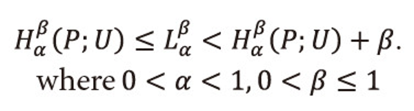
Theorem 3.1: Let <math xmlns="http://www.w3.org/1998/Math/MathML"> <mo>{</mo> <mi>u</mi> <mi>i</mi> <mo>}</mo> <mtable> <mtr> <mtd> <mi>n</mi> </mtd> </mtr> <mtr> <mtd> <mi>i</mi> <mo>=</mo> <mn>1</mn> </mtd> </mtr> </mtable> <mo>,</mo> <mo>{</mo> <mi>p</mi> <mi>i</mi> <mo>}</mo> <mtable> <mtr> <mtd> <mi>n</mi> </mtd> </mtr> <mtr> <mtd> <mi>i</mi> <mo>=</mo> <mn>1</mn> </mtd> </mtr> </mtable> </math>and <math xmlns="http://www.w3.org/1998/Math/MathML"> <mo>{</mo> <mi>l</mi> <mi>i</mi> <mo>}</mo> <mtable> <mtr> <mtd> <mi>n</mi> </mtd> </mtr> <mtr> <mtd> <mi>i</mi> <mo>=</mo> <mn>1</mn> </mtd> </mtr> </mtable> </math>, satisfies the inequality (2.14), then the two parametric generalized ‘useful’ code-word length (2.9) satisfies the inequality
Where <math xmlns="http://www.w3.org/1998/Math/MathML"> <msubsup> <mtext>H</mtext> <mtext>α</mtext> <mtext>β</mtext> </msubsup> </math>(P;U) and <math xmlns="http://www.w3.org/1998/Math/MathML"> <msubsup> <mtext>L</mtext> <mtext>α</mtext> <mtext>β</mtext> </msubsup> </math>(P;U) are defined in (2.1) and (2.9) respectively. Furthermore, equality holds good if
Proof: By Holder’s inequality, we have
For all xi, yi>0, i=1,2,3,…,n and <math xmlns="http://www.w3.org/1998/Math/MathML"> <mfrac> <mn>1</mn> <mi>p</mi> </mfrac> <mo>+</mo> <mfrac> <mn>1</mn> <mi>q</mi> </mfrac> <mo>=</mo> <mn>1</mn> </math>, p<1(≠0), q<0 or q<1(≠0), p<0. We see the equality holds if there exists a positive constant c such that
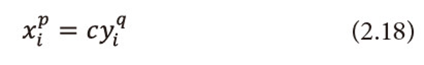
Making the substitution
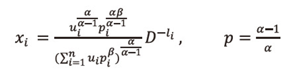
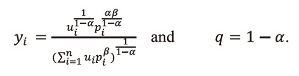
Using these values in (2.17), and after suitable simplification, we get
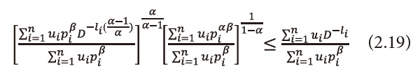
Now using the inequality (2.14), we get
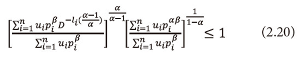
Or equation (2.20), can be written as
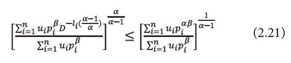
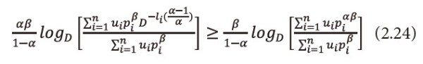
Taking logarithms to both sides with base D to equation (2.21), we get
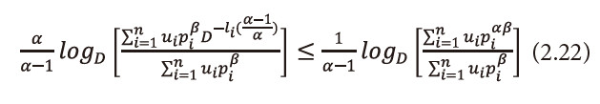
Or equivalently we can write equation (2.22), as
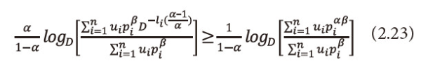
As 0<β≤1, multiply equation (2.23) both sides by β, we get
This implies

Hence the result for 0<α<1, 0<β≤1.
Now we will show that the equality in (2.15) holds if and only if
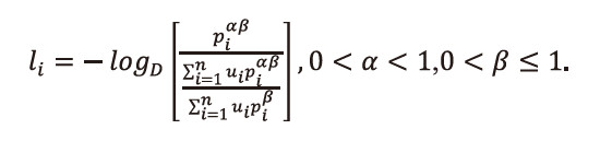
Or equivalently we can write
Or we can write
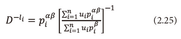
Raising both sides to the power <math xmlns="http://www.w3.org/1998/Math/MathML"> <mfrac> <mrow> <mtext>α</mtext> <mo>-</mo> <mn>1</mn> </mrow> <mtext>α</mtext> </mfrac> </math>, to equation (2.25), and after simplification we get
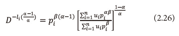
Multiply equation (2.26) both sides by
, and then summing over i=1,2,…,n, both sides to the resulted expression and after suitable simplification, we get
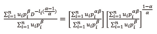
Or equivalently we can write
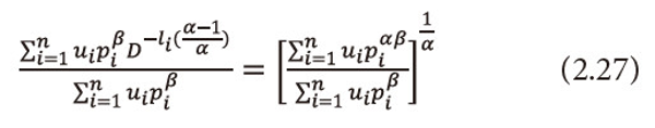
Taking logarithms both sides with base D to equation (2.27), then multiply both sides by <math xmlns="http://www.w3.org/1998/Math/MathML"> <mfrac> <mtext>αβ</mtext> <mrow> <mo>(</mo> <mn>1</mn> <mo>-</mo> <mtext>α</mtext> <mo>)</mo> </mrow> </mfrac> </math>, we get
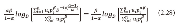
This implies
<math xmlns="http://www.w3.org/1998/Math/MathML"> <msubsup> <mtext>L</mtext> <mtext>α</mtext> <mtext>β</mtext> </msubsup> </math>(P;U) = <math xmlns="http://www.w3.org/1998/Math/MathML"> <msubsup> <mtext>H</mtext> <mtext>α</mtext> <mtext>β</mtext> </msubsup> </math>(P;U). Hence the result
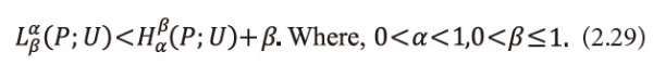
Theorem 3.2: For every code with lengths l1,l2,...,ln satisfies the condition (2.14), <math xmlns="http://www.w3.org/1998/Math/MathML"> <msubsup> <mtext>L</mtext> <mtext>α</mtext> <mtext>β</mtext> </msubsup> </math>(P;U) can be made to satisfy the inequality
Proof: From the theorem (2.1) we have
<math xmlns="http://www.w3.org/1998/Math/MathML"> <msubsup> <mtext>L</mtext> <mtext>α</mtext> <mtext>β</mtext> </msubsup> </math>(P;U) = <math xmlns="http://www.w3.org/1998/Math/MathML"> <msubsup> <mtext>H</mtext> <mtext>α</mtext> <mtext>β</mtext> </msubsup> </math>(P;U), holds if and only if
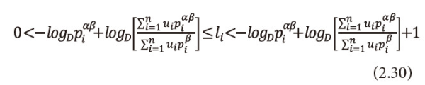
Now we choose the code-word lengths l1,l2,...,ln, in such a way that they satisfy the inequality,
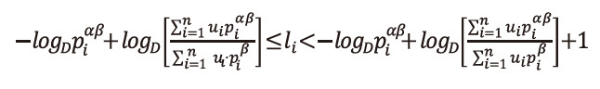
of length unity. In every <math xmlns="http://www.w3.org/1998/Math/MathML"> <mtext>δ</mtext> </math>i, there lies exactly one positive integer li, such that,
Now we will first show that the sequence l1,l2,...,ln, thus defined satisfies the inequality (2.14), which is a generalization of Kraft inequality.
From the left inequality of (2.30), we have
Or equivalently we can write
Multiply equation (2.31) both sides by then summing over i=1,2,…,n, both sides to the resulted expression, and after suitable operations, we get the required result (2.14), i.e.,
Now the last inequality of (2.30), gives
Or equivalently we can write
As 0<α<1, then(1-α)>0, and <math xmlns="http://www.w3.org/1998/Math/MathML"> <mfrac> <mrow> <mn>1</mn> <mo>-</mo> <mtext>α</mtext> </mrow> <mtext>α</mtext> </mfrac> </math> > 0, raising both sides to the power <math xmlns="http://www.w3.org/1998/Math/MathML"> <mfrac> <mrow> <mn>1</mn> <mo>-</mo> <mtext>α</mtext> </mrow> <mtext>α</mtext> </mfrac> </math> > 0, to equation (2.32), and after suitable operations, we get
Or equivalently we can write
Multiply equation (2.33) both sides by

, and then summing over i=1,2,…,n, both sides to the resulted expression and after suitable simplification, we get
Or equivalently we can write
Taking logarithms with base D both sides to the equation (2.34), we get
As 0<α<1,0<β≤1 then(1-α)>0 and <math xmlns="http://www.w3.org/1998/Math/MathML"> <mfrac> <mtext>αβ</mtext> <mrow> <mtext>1</mtext> <mo>-</mo> <mtext>α</mtext> </mrow> </mfrac> </math> >0, multiply equation (2.35), both sides by <math xmlns="http://www.w3.org/1998/Math/MathML"> <mfrac> <mtext>αβ</mtext> <mrow> <mtext>1</mtext> <mo>-</mo> <mtext>α</mtext> </mrow> </mfrac> </math> >0, we get
This implies
Hence the result for 0<α<1,0<β≤1.
Thus from above two coding theorems, we have shown that
In the next section we verify the noiseless coding theorems by considering the Shannon-Fano coding scheme and Huffman coding scheme by taking an empirical dataset.
4. ILLUSTRATION
In this section we illustrate the veracity of the theorems 3.1 and 3.2 by taking empirical data as given in Tables 1 and 2 on the lines of A. H. Bhat and M. A. K. Baig (2016).
Using Huffman coding scheme the values of <math xmlns="http://www.w3.org/1998/Math/MathML"> <msubsup> <mtext>H</mtext> <mtext>α</mtext> <mtext>β</mtext> </msubsup> </math>(P;U), <math xmlns="http://www.w3.org/1998/Math/MathML"> <msubsup> <mtext>H</mtext> <mtext>α</mtext> <mtext>β</mtext> </msubsup> </math>(P;U) + β, <math xmlns="http://www.w3.org/1998/Math/MathML"> <msubsup> <mtext>L</mtext> <mtext>α</mtext> <mtext>β</mtext> </msubsup> </math>(P;U) and η for different values of α and β are shown in the following Table 1.
Now using Shannon-Fano coding scheme the values of <math xmlns="http://www.w3.org/1998/Math/MathML"> <msubsup> <mtext>H</mtext> <mtext>α</mtext> <mtext>β</mtext> </msubsup> </math>(P;U), <math xmlns="http://www.w3.org/1998/Math/MathML"> <msubsup> <mtext>H</mtext> <mtext>α</mtext> <mtext>β</mtext> </msubsup> </math>(P;U) + β, <math xmlns="http://www.w3.org/1998/Math/MathML"> <msubsup> <mtext>L</mtext> <mtext>α</mtext> <mtext>β</mtext> </msubsup> </math>(P;U) and η for different values of α and β are shown in the following Table 2.
From Tables 1 and 2 we infer the following:
Ⅰ. Theorems 3.1 and 3.2 hold both the cases of Shannon-Fano codes and Huffman codes, i.e. <math xmlns="http://www.w3.org/1998/Math/MathML"> <msubsup> <mtext>H</mtext> <mtext>α</mtext> <mtext>β</mtext> </msubsup> </math>(P;U) ≤ <math xmlns="http://www.w3.org/1998/Math/MathML"> <msubsup> <mtext>L</mtext> <mtext>α</mtext> <mtext>β</mtext> </msubsup> </math>(P;U) < <math xmlns="http://www.w3.org/1998/Math/MathML"> <msubsup> <mtext>H</mtext> <mtext>α</mtext> <mtext>β</mtext> </msubsup> </math>(P;U) + β. where 0<α<1,0<β≤1.
Ⅱ. Huffman mean code-word length is less than Shannon-Fano mean code-word length.
Ⅲ. Coefficient of efficiency of Huffman codes is greater than coefficient of efficiency of Shannon-Fano codes; i.e., it is concluded that Huffman coding scheme is more efficient than Shannon-Fano coding scheme.
Table 1
Using Huffman coding scheme the values of <math xmlns="http://www.w3.org/1998/Math/MathML"> <msubsup> <mtext>H</mtext> <mtext>α</mtext> <mtext>β</mtext> </msubsup> </math>(P;U), <math xmlns="http://www.w3.org/1998/Math/MathML"> <msubsup> <mtext>H</mtext> <mtext>α</mtext> <mtext>β</mtext> </msubsup> </math>(P;U)+β, <math xmlns="http://www.w3.org/1998/Math/MathML"> <msubsup> <mtext>L</mtext> <mtext>α</mtext> <mtext>β</mtext> </msubsup> </math>(P;U) and η for different values of α and β
| Probabilities Pi | Huffman Codewords | li | ui | α | β | Hαβ(P;U) | Lαβ(P;U) | η=Hαβ(P;U)/Lαβ(P;U) x 100 | Hαβ(P;U)+β |
|---|---|---|---|---|---|---|---|---|---|
| 0.41 | 1 | 1 | 6 | 0.9 | 1 | 1.987 | 2.012 | 98.757% | 2.987 |
| 0.18 | 000 | 3 | 5 | 0.9 | 0.9 | 1.654 | 1.874 | 88.260% | 2.554 |
| 0.15 | 001 | 3 | 1 | 0.8 | 1 | 2.016 | 2.079 | 96.969% | 3.016 |
| 0.13 | 010 | 3 | 2 | ||||||
| 0.1 | 0110 | 4 | 4 | ||||||
| 0.03 | 0111 | 4 | 3 |
Table 2
Using Shannon-Fano coding scheme the values of <math xmlns="http://www.w3.org/1998/Math/MathML"> <msubsup> <mtext>H</mtext> <mtext>α</mtext> <mtext>β</mtext> </msubsup> </math>(P;U), <math xmlns="http://www.w3.org/1998/Math/MathML"> <msubsup> <mtext>H</mtext> <mtext>α</mtext> <mtext>β</mtext> </msubsup> </math>(P;U)+β, <math xmlns="http://www.w3.org/1998/Math/MathML"> <msubsup> <mtext>L</mtext> <mtext>α</mtext> <mtext>β</mtext> </msubsup> </math>(P;U) and η for different values of α and β
| Probabilities Pi | Shannon-Fano<br>Codewords | li | ui | α | β | Hαβ(P;U) | Lαβ(P;U) | η=Hαβ(P;U)/Lαβ(P;U) x 100 | Hαβ(P;U)+β |
|---|---|---|---|---|---|---|---|---|---|
| 0.41 | 00 | 2 | 6 | 0.9 | 1 | 1.987 | 2.217 | 89.625% | 2.987 |
| 0.18 | 01 | 2 | 5 | 0.9 | 0.9 | 1.654 | 2.014 | 82.125% | 2.554 |
| 0.15 | 100 | 3 | 1 | 0.8 | 1 | 2.016 | 2.226 | 90.566% | 3.016 |
| 0.13 | 101 | 3 | 2 | ||||||
| 0.1 | 110 | 3 | 4 | ||||||
| 0.03 | 111 | 3 | 3 |
5. MONOTONIC BEHAVIOR OF THE TWO PARAMETRIC NEW GENERALIZED ‘USEFUL’ INFORMATION MEASURE <math xmlns="http://www.w3.org/1998/Math/MathML"> <msubsup> <mtext>H</mtext> <mtext>α</mtext> <mtext>β</mtext> </msubsup> </math>(P;U)
In this section we study the monotonic behavior of the new two parametric generalized ‘useful’ information measure <math xmlns="http://www.w3.org/1998/Math/MathML"> <msubsup> <mtext>H</mtext> <mtext>α</mtext> <mtext>β</mtext> </msubsup> </math>(P;U) given in (2.1) with respect to the parameters α and β.
Let P=(0.41, 0.18, 0.15, 0.13, 0.10, 0.03) be a set of probabilities. Assuming β=1 we calculate the values of <math xmlns="http://www.w3.org/1998/Math/MathML"> <msubsup> <mtext>H</mtext> <mtext>α</mtext> <mtext>β</mtext> </msubsup> </math>(P;U) for different values of α as shown in the following Table 3.
Next we draw the graph of the table (3) and illustrate from Figure 1 that <math xmlns="http://www.w3.org/1998/Math/MathML"> <msubsup> <mtext>H</mtext> <mtext>α</mtext> <mtext>β</mtext> </msubsup> </math>(P;U) is monotonic decreasing with increasing values of α.
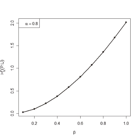
Now assuming α=0.8 we calculate the values of <math xmlns="http://www.w3.org/1998/Math/MathML"> <msubsup> <mtext>H</mtext> <mtext>α</mtext> <mtext>β</mtext> </msubsup> </math>(P;U) for different values of β as shown in the following Table 4.
Next we draw the graph of the table (4) and illustrate from Figure 2 that <math xmlns="http://www.w3.org/1998/Math/MathML"> <msubsup> <mtext>H</mtext> <mtext>α</mtext> <mtext>β</mtext> </msubsup> </math>(P;U) is monotonic increasing with increasing values of β.
Table 3
Monotonic Behavior of <math xmlns="http://www.w3.org/1998/Math/MathML"> <msubsup> <mtext>H</mtext> <mtext>α</mtext> <mtext>β</mtext> </msubsup> </math>(P;U) with Respect to α for fixed β=1
| α | 0.1 | 0.2 | 0.3 | 0.4 | 0.5 | 0.6 | 0.7 | 0.8 | 0.9 |
|---|---|---|---|---|---|---|---|---|---|
| Hαβ(P;U) | 2.260 | 2.221 | 2.2.182 | 2.146 | 2.112 | 2.078 | 2.047 | 2.017 | 1.988 |
Fig. 1
Monotonic behavior of <math xmlns="http://www.w3.org/1998/Math/MathML"> <msubsup> <mtext>H</mtext> <mtext>α</mtext> <mtext>β</mtext> </msubsup> </math>(P) with respect to α for fixed β=1
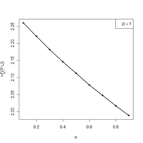
Table 4
Monotonic Behavior of <math xmlns="http://www.w3.org/1998/Math/MathML"> <msubsup> <mtext>H</mtext> <mtext>α</mtext> <mtext>β</mtext> </msubsup> </math>(P;U) with Respect to β for fixed α=0.8
| β | 0.1 | 0.2 | 0.3 | 0.4 | 0.5 | 0.6 | 0.7 | 0.8 | 0.9 | 1 |
|---|---|---|---|---|---|---|---|---|---|---|
| Hαβ(P;U) | 0.026 | 0.102 | 0.222 | 0.383 | 0580 | 0.811 | 1.072 | 1.361 | 1.677 | 2.017 |
Fig. 2
Monotonic behavior of <math xmlns="http://www.w3.org/1998/Math/MathML"> <msubsup> <mtext>H</mtext> <mtext>α</mtext> <mtext>β</mtext> </msubsup> </math>(P;U) with respect to β for fixed α=0.8
6. PROPERTIES OF THE NEW TWO PARAMETRIC GENERALIZED ‘USEFUL’ INFORMATION MEASURE <math xmlns="http://www.w3.org/1998/Math/MathML"> <msubsup> <mtext>H</mtext> <mtext>α</mtext> <mtext>β</mtext> </msubsup> </math>(P;U)
In this section we will discuss some properties of the two parametric new generalized ‘useful’ information measure <math xmlns="http://www.w3.org/1998/Math/MathML"> <msubsup> <mtext>H</mtext> <mtext>α</mtext> <mtext>β</mtext> </msubsup> </math>(P;U) given in (2.1):
Property 6.1: <math xmlns="http://www.w3.org/1998/Math/MathML"> <msubsup> <mtext>H</mtext> <mtext>α</mtext> <mtext>β</mtext> </msubsup> </math>(P;U) is non-negative.
Proof: From (2.1), we have
From Tables 1 and 2, it is observed that <math xmlns="http://www.w3.org/1998/Math/MathML"> <msubsup> <mtext>H</mtext> <mtext>α</mtext> <mtext>β</mtext> </msubsup> </math>(P;U) is non-negative for given values of α and β.
Property 6.2: <math xmlns="http://www.w3.org/1998/Math/MathML"> <msubsup> <mtext>H</mtext> <mtext>α</mtext> <mtext>β</mtext> </msubsup> </math>(P;U) is a symmetric function on every pi, i=1,2,3,…,n.
Proof: It is obvious that <math xmlns="http://www.w3.org/1998/Math/MathML"> <msubsup> <mtext>H</mtext> <mtext>α</mtext> <mtext>β</mtext> </msubsup> </math>(P;U) is a symmetric function on every pi, i=1,2,3,… ,n.i.e., <math xmlns="http://www.w3.org/1998/Math/MathML"> <msubsup> <mtext>H</mtext> <mtext>α</mtext> <mtext>β</mtext> </msubsup> </math>(p1u1,p2u2,...,pn-1un-1,pnun) = <math xmlns="http://www.w3.org/1998/Math/MathML"> <msubsup> <mtext>H</mtext> <mtext>α</mtext> <mtext>β</mtext> </msubsup> </math>(pnun,p1u1,p2u2,...,pn-1un-1)
Property 6.3: <math xmlns="http://www.w3.org/1998/Math/MathML"> <msubsup> <mtext>H</mtext> <mtext>α</mtext> <mtext>β</mtext> </msubsup> </math>(P;U) is maximum when all the events have equal probabilities.
Proof: When pi = <math xmlns="http://www.w3.org/1998/Math/MathML"> <mfrac> <mn>1</mn> <mi>n</mi> </mfrac> <mo>∀</mo> <mi>i</mi> </math> = 1,2,...,n and β=1,α→1. and ui = 1, <math xmlns="http://www.w3.org/1998/Math/MathML"> <mo>∀</mo> <mi>i</mi> </math> = 1,2,...,n, i.e., when the utility aspect is ignored, <math xmlns="http://www.w3.org/1998/Math/MathML"> <msubsup> <mtext>Σ</mtext> <mrow> <mi>i</mi> <mo>=</mo> <mn>1</mn> </mrow> <mi>n</mi> </msubsup> </math>pi=1. Then <math xmlns="http://www.w3.org/1998/Math/MathML"> <msubsup> <mtext>H</mtext> <mtext>α</mtext> <mtext>β</mtext> </msubsup> </math>(P;U) = logDn, which is maximum entropy.
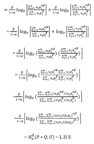
Property 6.4: <math xmlns="http://www.w3.org/1998/Math/MathML"> <msubsup> <mtext>H</mtext> <mtext>α</mtext> <mtext>β</mtext> </msubsup> </math>(P;U) satisfies the additivity of the following form:
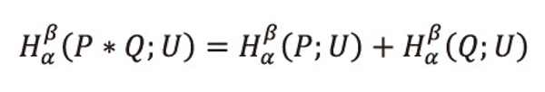
Where (P*Q:U)=(p1q1,...,p1qm,p2q1,...,p2qm,...,pnq1,...,pnqm;U)
Proof: Let <math xmlns="http://www.w3.org/1998/Math/MathML"> <msubsup> <mtext>H</mtext> <mtext>α</mtext> <mtext>β</mtext> </msubsup> </math>(P*Q;;U) = <math xmlns="http://www.w3.org/1998/Math/MathML"> <msubsup> <mtext>H</mtext> <mtext>α</mtext> <mtext>β</mtext> </msubsup> </math>(P;U) + <math xmlns="http://www.w3.org/1998/Math/MathML"> <msubsup> <mtext>H</mtext> <mtext>α</mtext> <mtext>β</mtext> </msubsup> </math>(Q;U)
Taking R.H.S= <math xmlns="http://www.w3.org/1998/Math/MathML"> <msubsup> <mtext>H</mtext> <mtext>α</mtext> <mtext>β</mtext> </msubsup> </math>(P;U) + <math xmlns="http://www.w3.org/1998/Math/MathML"> <msubsup> <mtext>H</mtext> <mtext>α</mtext> <mtext>β</mtext> </msubsup> </math>(Q;U)
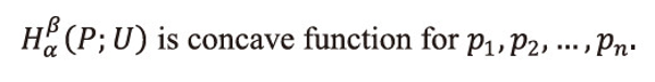
Property 6.5: <math xmlns="http://www.w3.org/1998/Math/MathML"> <msubsup> <mtext>H</mtext> <mtext>α</mtext> <mtext>β</mtext> </msubsup> </math>(P) is concave function for p1,p2,...,pn.
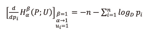
Proof: From (2.1), we have
If β=1, α→1, ui=1, ∀i=1,2,...,n, i.e., when the utility aspect is ignored, and <math xmlns="http://www.w3.org/1998/Math/MathML"> <msubsup> <mtext>Σ</mtext> <mrow> <mi>i</mi> <mo>=</mo> <mn>1</mn> </mrow> <mi>n</mi> </msubsup> </math>pi=1. then the first derivative of (2.1) with respect is given by
And the second derivative is given by
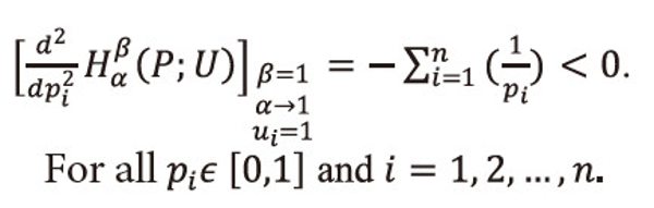
Since the second derivative of <math xmlns="http://www.w3.org/1998/Math/MathML"> <msubsup> <mtext>H</mtext> <mtext>α</mtext> <mtext>β</mtext> </msubsup> </math>(P;U) with respect to pi is negative on given interval pi <math xmlns="http://www.w3.org/1998/Math/MathML"> <mtext>ε</mtext> </math>[0,1], i=1,2,…,n. as β=1, α→1, ui=1, ∀i=1,2,...,n, i.e., when the utility aspect is ignored, and <math xmlns="http://www.w3.org/1998/Math/MathML"> <msubsup> <mtext>Σ</mtext> <mrow> <mi>i</mi> <mo>=</mo> <mn>1</mn> </mrow> <mi>n</mi> </msubsup> </math>pi=1, therefore,
7. CONCLUSION
In this paper we define a new two parametric generalized ‘useful’ entropy measure, i.e., <math xmlns="http://www.w3.org/1998/Math/MathML"> <msubsup> <mtext>H</mtext> <mtext>α</mtext> <mtext>β</mtext> </msubsup> </math>(P;U). This measure also generalizes some well-known information measures already existing in the literature of ‘useful’ information theory. Also we define a new two parametric generalized ‘useful’ code-word mean lengths, i.e., <math xmlns="http://www.w3.org/1998/Math/MathML"> <msubsup> <mtext>L</mtext> <mtext>α</mtext> <mtext>β</mtext> </msubsup> </math>(P;U) corresponding to <math xmlns="http://www.w3.org/1998/Math/MathML"> <msubsup> <mtext>H</mtext> <mtext>α</mtext> <mtext>β</mtext> </msubsup> </math>(P;U), and then we characterize <math xmlns="http://www.w3.org/1998/Math/MathML"> <msubsup> <mtext>L</mtext> <mtext>α</mtext> <mtext>β</mtext> </msubsup> </math>(P;U) in terms of <math xmlns="http://www.w3.org/1998/Math/MathML"> <msubsup> <mtext>H</mtext> <mtext>α</mtext> <mtext>β</mtext> </msubsup> </math>(P;U) and showed that
Further we have established the noiseless coding theorems proved in this paper with the help of two different techniques by taking experimental data and showed that Huffman coding scheme is more efficient than Shannon-Fano coding scheme. We have also studied the monotonic behavior of <math xmlns="http://www.w3.org/1998/Math/MathML"> <msubsup> <mtext>H</mtext> <mtext>α</mtext> <mtext>β</mtext> </msubsup> </math>(P;U) with respect to parameters α and β. The important properties of <math xmlns="http://www.w3.org/1998/Math/MathML"> <msubsup> <mtext>H</mtext> <mtext>α</mtext> <mtext>β</mtext> </msubsup> </math>(P;U) have also been studied.
- 투고일Submission Date
- 2016-07-03
- 수정일Revised Date
- 게재확정일Accepted Date
- 2016-11-28
- 480다운로드 수
- 949조회수
- 0KCI 피인용수
- 0WOS 피인용수